

How to Flip the Sign on Feedbacks
For context I strongly recommend reading (and understanding!) those two articles first:
A Falsification - the incredibly stupid case of water vapor feedback
The Climate Kill Switch – Why Feedbacks are Actually Negative
As always, basic climate physics is kind of hidden away in climate models, which are pretty inaccessible to the outside world, but even the “climate experts” playing with these models might not actually know about the innards. Writing the code (in the back end) and publishing model output are two different things. Anyway, once you know about the physics the models try to emulate, published model outputs will provide valuable insights.
I found three illustrations of lapse rate feedback (LRF) online, as listed below. They are based on different models and they have different scales. One is north to south in the x-scale and has the poles inverted, while the one in the middle uses a surface area weighted scale (=sin(latitude)). Note that 50% of the Earths surface is in the tropical range between 30° latitude north and south respectively.
Klocke et al 20131
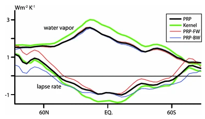
Beer et al 20222
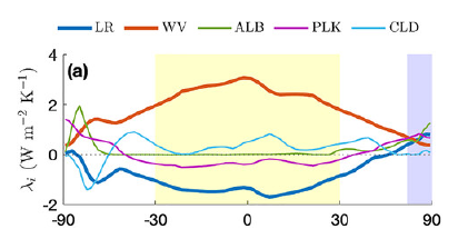
Pithan et al 20133
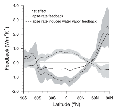
They all look similar, with the main negative part of the lapse rate feedback located in the tropical range of about -1.2W/m2, +/- something. I did some point for point analysis with the last graph and found that is would correspond to a total LRF of -0.62 which is on the higher end of current LRF estimates (typically in the -0.5 to -0.6 range). The one in the middle gives an even higher figure of above -0.8W/m2, consistent with the central AR4 estimate of -0.84.
There seems to be a basic relation between tropical and global LRF in the models of about 2. If it is like -1W/m2 in the tropics, it will be about -0.5 globally, or like -1.7 to -0.85, but that basic relation is pretty stable.
Let’s recapitulate the evolution here since AR4:
In AOGCMs, the water vapour feedback constitutes by far the strongest feedback, with a multi-model mean and standard deviation for the MMD at PCMDI of 1.80 ± 0.18 W m–2 °C–1, followed by the (negative) lapse rate feedback (–0.84 ± 0.26 W m–2 °C–1) and the surface albedo feedback (0.26 ± 0.08 W m–2 °C-1). The cloud feedback mean is 0.69 W m–2 °C–1 with a very large inter-model spread of ±0.38 W m–2 °C–1 (Soden and Held, 2006).
AR5:
We estimate the water vapour plus lapse rate feedback to be +1.1 (+0.9 to +1.3) W m−2 °C−1
AR6:
The LR feedback has been estimated at interannual time scales using meteorological reanalysis and satellite measurements of TOA fluxes (Dessler, 2013). These estimates from climate variability are consistent between observations and ESMs (Dessler, 2013; Colman and Hanson, 2017). The mean and standard deviation of this feedback under global warming based on the cited studies are αLR = –0.50 ± 0.20 W m–2 °C –1
Since AR5 it has been clarified that by construction, the sum of the temperature lapse rate and specific humidity (LR + WV) feedbacks is equal to the sum of the Clausius Clapeyron feedback
The CC feedback has a large positive value due to well understood thermodynamic and radiative processes: αCC = 1.36 ± 0.04 W m–2 °C–1
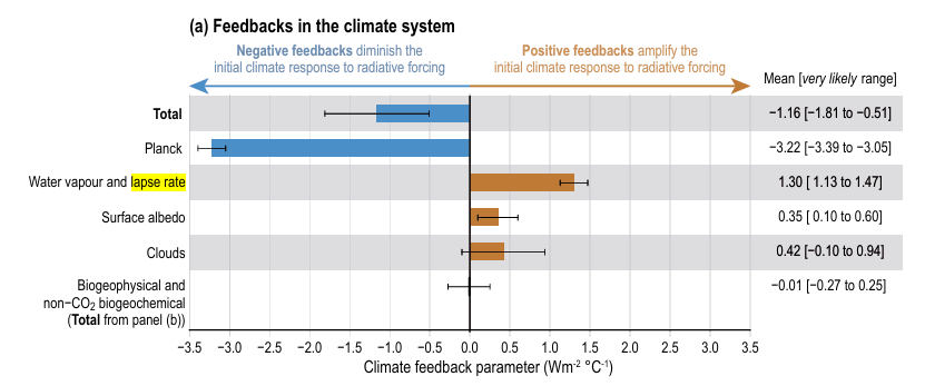
It remains a bit ambiguous whether the central estimate on the combined water vapor and lapse rate feedback is 1.3, or even 1.36 in AR6. I mean given it is central estimate anyhow, some uncertainty should be conceded. The point is, this figure has grown substantially since AR4. The combined term was 0.96 (=1.8-0.84) back then, grew to 1.1 with AR5, and now stands at say 1.3. It sums up to a 0.34W/m2 feedback increment (or even 0.4 if we would assume the 1.36 “CC feedback”), entirely due to reducing the LRF.
It is easy to show what impact this will have on climate sensitivity. Despite there still being a lot of uncertainty, we can just pick an exemplary central estimate to demonstrate the effect, with 3.7W/m2 for 2xCO2 forcing, 0.3 as lambda (the inverted Planck Response or “Planck Feedback”) and 2W/m2 as the initial sum of feedbacks.
3.7 * 0.3 / (1 - 2 * 0.3) = 2.775
3.7 * 0.3 / (1 - 2.34 * 0.3) = 3.725
The reduction of the LRF estimate is the one reason why climate sensitivity went up, by almost 1K in this instance. It would be (substantially) more with higher base feedback assumptions, and less in the opposite case. Yet it is the factor that drove the ECS range higher, from 1.5 to 4.5 to now 2.5 to 4K, with the central estimate though still remaining at 3K.
Of course it might seem somewhat counterintuitive, as the reduction of negative LRF will simply result in larger overall feedbacks, thereby not just increasing ECS, but also the range of uncertainty. But these figures are just roughly rounded “communication estimates”, to be taken with a lot of salt. Also the central estimate was actually 2.5K with the first two assessment reports. And while there has been quite some discussion of this gradual ECS increment, the main cause, the reduction of LRF, was not named, at least not in the articles I read.
The Tropical Lapse Rate
Now what I actually wanted to discuss is the argument brought up, the (negative) lapse rate feedback was mainly a thing of the tropics and offset by a positive LRF in high latitudes. I have a lot of issues with that, for different reasons, but why not have a closer look at the tropics and the “hot spot” there. Here we have a model output posted on realclimate4.
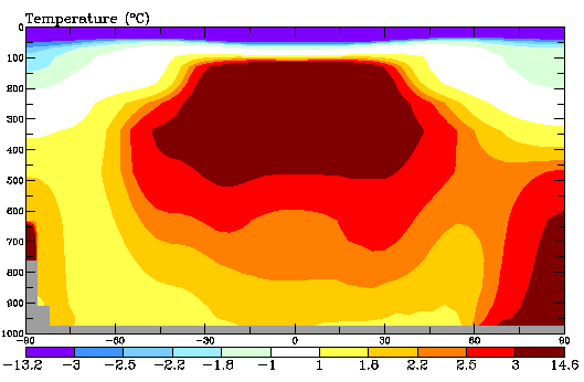
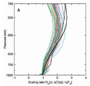
In the text hereto it states “It’s important to note however, that these are long-term equilibrium results”. That is indeed an important detail, distinguishing it from the Santer et al 20055 (S05) chart on the tropical lapse rate below, which shows a transient model output, where ocean temperature is lagging behind and (most) models have a lesser decrease of the lapse rate as in long-term theory.
Although we have to guess a bit, the realclimate chart would suggest some 1.8K of surface warming in the tropics, or maybe somewhat less. Please note the graph has greyed out the lowest ~250m. If it was not for that, the whole surface would be in the yellow range, somewhere between 1 to 1.8K, though certainly to the higher end, in the tropics. From about 500mbar upward it is all deep red, meaning at least 3K of warming.
Now in the tropics the average emission altitude is somewhat higher, roughly over 6km altitude at a pressure level of around 450mbar. With these values we can infer an increment of Tz at least 1.67times (=3/1.8) larger than that of Ts, though in that specific model it might even be 2times, like 3.2/1.6.
If we assume a black body emission temperature of 260K in the tropics, we can make some basic calculations based on the Stefan-Boltzmann law.
((260 + 1.67)^4 - 260^4 * 5.67e-8) = -6.72
Or alternatively..
((260 + 2)^4 - 260^4 * 5.67e-8) = -8.05
Either way, whatever scenario one assumes exactly, the amount of outgoing longwave radiation (OLR) in response to a 1K increment of surface temperature is massive. It is the one thing totally evident to anyone who even slightly understands physics, when looking at that “hot spot” graph. This is where the planet loses energy into space, and the warmer that part is, the more efficient that cooling.
It is virtually like a heat sink. If you have a CPU consuming a 100Watt of energy on a tiny space, you need to cool it, or it will just melt away. So we put a heat sink on it to absorb that heat, we give it a lot of surface area and then have a fan blowing air on it all, so that heat can dissipate. You will want to move the heat from where it is contained to a place where it can dissipate. And that is exactly what that “hot spot” is about, it concentrates the heat where it can escape to space. But while there is a lot of (incompetent) talk over the greenhouse effect, you will never have heard about that heat sink effect. Yet it is real.
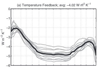
As above, the combination of Planck Response and LRF is sometimes referred to in the literature as “temperature feedback”, like in Zelinka, Hartmann 20116 (ZH11). That is a very helpful as an alternative perspective, because then WV and LR feedback are no more coupled, and we do not even need to discuss the issues “consensus science” has with the Planck response. Rather it all boils down to simple physics.
I should also introduce you to another perspective on climate sensitivity as named in ZH11:
The sum of all feedbacks when integrated over the entire planet is -1 W m−2 K−1, indicating a climate that is stable to perturbations, though significantly less stable than a blackbody planet with no atmospheric feedbacks other than the basic Planck feedback of about 3.2 W m−2 K−1
This might sound very confusing, because feedbacks then were negative all over(!?), but in this metric though they simply have to be. What they do in this instance is to count the Planck Response as a negative feedback (be it part of temperature feedback) and then add up all the feedbacks. It is a simple calculation..
-4.02 Temperature Feedback
0.61 Cloud Feedback
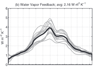
2.16 Water Vapor Feedback
0.27 Albedo Feedback
---------------------------------
-0.98 Total Feedback
It translates into this: if there is one Kelvin of warming at the surface, only an additional 0.98W/m2 will leave the system. Eventually you would relate this total negative feedback to a positive forcing, like a 3.7W/m2 you might get from a doubling of CO2. The ECS then is 3.7/0.98 = 3.7755K. Although it may all sound unfamiliar, it is still the very same bottom line that “consensus science” is all about. Of course you would get the same result with..
(3.7 / 3.2) / (1 - (0.61 + 2.16 + 0.27 - 0.82) / 3.2) = 3.7755
Interestingly it will not even matter how exactly you split up the temperature feedback. Above it is 3.2 and 0.82 respectively, but for instance 3 and 1.02 would yield the identical result..
(3.7 / 3) / (1 - (0.61 + 2.16 + 0.27 - 1.02) / 3) = 3.7755
It is all just number games. What factors cause an increment in OLR will not matter, and so there is indeed no material difference between the Planck Response and Lapse Rate Feedback. Physically they have the very same effect and the math representing said physics, will not discriminate. It is all straight forward and logic.
The interesting part about this perspective is over the fragility of that -0.98 figure, making it instantly evident how important the Planck Response, or rather the assessment hereto is. If it was -3.2W/m2 as in the quote above, that would leave still -0.82W/m2 remainder for the lapse rate feedback. Please remember TH11 was published in, you name it, 2011 when AR4 was the latest consensus position by the IPCC, which had LRF at -0.84 as a central estimate. The relatively high ECS here did not come from understating the LRF, but rather from overstating WVF with 2.16W/m2, as opposed to a central 1.8W/m2 in AR4.
In the tropics the ZH11 chart suggests about ~4.85W/m2 temperature feedback, within a range of 4 to 5.6. If we assume an emission temperature of 260K within the tropics, we can derive the change in the emission temperature. With t1 being the new emission temperature and tf the temperature feedback, formula would go like..
(t1^4 - 260^4) * 5.67e-8 = tf
Solving for t1 will give us..
t1 = (tf / 5.67e-8 + 260^4)^0.25
For the respective range of tf (min, mean, max) we get..
4.0…. 261
4.85.. 261.21
5.6… 261.39
Relative to Ts, the emission temperature would increase by 21%, with a range of 0 to 39%.
Considering the Stratosphere
Now one also might want to consider the stratosphere. As we all know the stratosphere will cool with the addition of CO2, because there will be more emitting stuff. As the stratosphere holds a small share in OLR, one could assume this being a kind of positive lapse rate feedback, partially offsetting what goes on in the troposphere. The thing is though, just because the stratosphere cools, will not mean it would also emit less into space.
If we doubled stratospheric CO2 at once, due to the increment in optical thickness, it would rather emit more in the first place and only then the consequent cooling offsets this effect, bringing things back into balance. Unless the amount of energy absorbed changes, the stratosphere will emit just the same, regardless how much CO2 there is.
But there is yet another interesting detail. With a higher optical thickness, the stratosphere will also absorb more terrestrial IR from below. So one could think like this; if there is more energy emitted into space but also (actually proportionally) more absorbed from down below, would that not cancel out? And if so, why would the stratosphere cool? But then you would forget about the stratosphere also emitting more downward, which already neutralizes the additional LWIR absorption. Again, that part is a zero-sum game, not doing anything. You would be confusing radiative exchange with an input (or loss) of energy, bringing us back to the whole “back radiation” nonsense. Anyway..
Yet the stratosphere does make a difference in the way that it absorbs a fraction of the upwelling radiation. In the tropical modtran scenario at an altitude of 17km, roughly the tropopause there, downwelling radiation would amount to 9.7W/m2. The OLR from the stratosphere then should be gradually larger, because it gets warmer with altitude, but it should remain within a 4% of the total OLR (>9.7/260). I will skip a more detailed discussion. The point is, the tropospheric temperature feedback should get attenuated by about 4% just because the stratosphere, so to say, stands in the way. We can incorporate this detail in the above formula and it will change the outcome slightly, by said 4%..
(t1^4 - 260^4) * 5.67e-8 * 0.96 = tf
For the respective tf ranges you then get..
4.0… 261.04
4.85.. 261.26
5.6… 261.45
It is bit more than before, but it will not solve the underlying problem. If you want to argue large climate sensitivity, you will have to maximize all positive feedbacks, AND minimize the negative feedbacks, it is as simple as that. Whether it is the Planck Response or LRF, you would want to minimize both of them. As the temperature feedback consists of both these two, it kind of holds the essence of said attempt so that both margins of “cutting all corners” accumulate.
The Different Versions of Temperature Feedback
For the sake of illustration I have projected these numbers onto the S05 chart - in blue. I know, it is simplified, it does not feature any specific curves, but it provides the proper dimensions. Also I am not sure what kind of scale they used. It seems to be logarithmic with regard to the pressure level, but might be linear in terms of altitude, but checking that out reveals it will not quite fit either. Whatever..
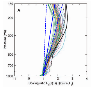
That difference is just irreconcilable and this conflict is directly affecting climate sensitivity. In this graph, in theory, the troposphere would warm between 1 and 2.7K, with the average emission temperature going up by about 1.8K, but definitely not 1.26, nor 1.45, the upper with the ZH11 model runs.
(261.8^4 - 260^4) * 5.67e-8 * 0.96 = 6.96
So like this we have a tropical temperature feedback of 6.96W/m2, +/- whatever, a gap of over 2W/m2 over the central model estimate. The gap is large enough to flip large positive feedback into no (positive) feedbacks at all. And that contradiction could not be more evident. I mean you can not postulate the troposphere warming at an according rate, but then deny the necessary physical consequences. Equally you can not rely on a theory, while at same time denying it.
We can try to break it down into its components. If the global Planck response was 3.2, as stated in ZH11, the tropical figure would be slightly larger, like 3.5 to 3.6. Let us assume the latter. Then the range of LRF there will be 0.4/1.25/2 (min, mean, max, =4-3.6, 4.85-3.6, 5.6-3.6)), pretty consistent with the sources presented at the beginning of this article. One problem is, the Planck response has to be ~3.85 under consideration of the stratosphere..
(261^4 - 260^4) * 5.67e-8 * 0.96 = 3.85
But then we are still left with a remainder of 3.11W/m2 (6.96-3.85) for real, which is LRF. And if we assumed a Planck Response of only 3.6, the remainder would be 3.36, a long shot from the range in the models. It remains an unforgiving contradiction, where both, Planck Response AND LRF, have been tuned down against better knowledge, just to push climate sensitivity up. And it is not a marginal thing either, but rather could not be more substantial.
If you look at fig.3 in ZH11 the tropical feedbacks are like known -4.85 temperature feedback, approx +1 cloud feedback and let us say +3.2 WV feedback, while albedo feedback is basically a flat zero in the tropics. If we sum this up we get about -0.65 for total feedbacks, roughly consistent with the sum of all feedbacks as in the chart below.
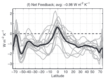
Notably in the inner tropics that sum would even turn positive, something referred to as the “super greenhouse effect” in the literature7. It is not just materially wrong, as discussed before, but also a mathematical absurdity. It does not matter how you put it, but in this context you would define F + ECS*NF = 0, with F being forcing and NF the net feedbacks and ‘0’ suggesting the equilibrium. Then ECS = -F/NF. That works with a negative net feedback of say -0.98, because -3.7/-0.98 = 3.775, as above. But if we assumed an NF of +0.5, we would get ECS = -3.7/0.5 = -7.4 in the inner tropics. In other words, there would be massive cooling?!
But now looking at the whole of the tropics, the -0.65 would be met not quite with a 3.7W/m2 forcing, but rather a bit more, like 4.1 to 4.2. CO2 forcing is simply larger in low latitudes with warm temperatures than in high latitudes. That is why some argue CO2 forcing would even be negative in Antarctica89, although that is not true either. Anyway, within the climate model world the tropics are so to say the heat engine, responsible for the bulk of climate sensitivity.
-4.2 / -0.65 = 6.5K
This is actually a somewhat complicated narrative. Although most of the warming would be generated in the tropics, the actual surface warming should behave exactly the opposite. Most warming should occur at the poles, thanks to polar amplification, while the tropics are quite resilient. The meridional heat transport would be very busy. And although it will be a problem, it is probably a minor one within the consensus narrative. Way more serious is the issue we get from substituting temperature feedback with our more accurate -6.96W/m2. Then..
-4.2 / (-6.96 + 1 + 3.2) = 1.52K
In words: not 6.5 but only 1.5K of climate sensitivity in the tropics. Just correcting that one obvious blunder with the temperature feedback, lets climate sensitivity collapse. The tropics turn from the driver to the brakeman of “climate change”.
Water Vapor
Tropical Water Vapor Feedback (WVF) on the other side is massive in the models. There is some difference between the inner- and the (dry) outer tropics. As in ZH11 it is up to 3.8 or 3.9 maximum in the inner tropics and about 3 in the outer tropics, with roughly +/-1 variability over the different model runs.
Let us check this against modtran10. There the inner tropical scenario yields a WVF of 1.727W/m2 (=303.858-302.131), which honestly does not mean a lot and must not be taken at face value. We have to sort out the details, the features and limitations of modtran first.
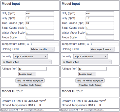
This is indeed an inner tropical scenario with about 51mm of precipitable water in the atmosphere. You can find that by checking out the “raw model output”. Then I am using a temperature offset of 1K and let modtran do the calculations according to the Clausius Clapeyron equation, which is more accurate than simply adding a certain percentage of WV, and yields a higher result (it would be 1.633 with a plain 7% increment). You can do that by switching between “Water Vapor Pressure” and “Relative Humidity”. Also I am using an altitude of only 17km so that we skip the whole stratosphere, which modtran would otherwise heat by equally 1K, making little sense in real life.
Yet there are two main issues left. For one that is with clear skies and we know adding clouds will sharply reduce the outcome. With the 3km cloud top scenario (Altostratus Clouds..) it is only 0.973W/m2 of WVF. Please note how a large share of the WVF in this case comes from low altitudes <3km, namely about 44% (= 1 - 0.973 / 1.727), which will be important in a moment. How to properly emulate clouds in modtran, or rather with modtran, beyond the far too simplistic scenarios it offers out of the box, is a separate discussion we already had. Generally one could assume a reduction of atmospheric forcings or feedbacks by about 30%, when introducing clouds into a clear sky base scenario. This would hold for the global average, but not for the inner tropics, where clouds are just more abundant.
Essentially with the help of modtran, you would conclude ~1W/m2 (likely less) WVF within in the inner tropics, under consideration of clouds and their overlaps with WV. But then of course there is the gorilla in the room, which is the lapse rate again. Regrettably modtran simply holds the lapse rate fixed, in troposphere but also beyond. So if you add 1K of surface temperature, it just shifts the whole thing right, meaning a linear warming of the whole atmosphere. Because of this, it can neither emulate the effect of LRF, nor properly model WVF itself. As much as the troposphere warms more than the surface, it can also hold additional WV and generate an accordingly larger WVF.
Btw. it should really not be too hard to add lapse rate effects to modtran and I want to believe it has been done a long time ago. However, the result would be just what I am pointing out here, that is a minimal climate sensitivity, in total contradiction of the consensus narrative. So you can be certain it will not ever be made accessible to the public. I digress..
In the outer tropics, because of a lower WV concentration in the first place, clear sky WVF is smaller anyway, like about 1.3W/m2. But there is a little issue with modtran. If you just half the “water vapor scale”, thereby effectively tuning down relative humidity and approximating the dry outer tropics, you get 1.57W/m2, again without clouds. This figure is way too high and a glitch due to limited resolution.
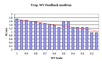
And it is just one approach to get some more out of modtran, by not just accepting the nominal figure, but also putting it into context. One can see pretty well the glitch around 0.5, and the very finite resolution to the right. By extrapolation of the results, checking back against other scenarios, the figure should be about 1.3W/m2. But just because the atmosphere is much dryer, of course there are also fewer clouds attenuating that figure. It should equally be about 1W/m2 for the “all sky” reality, maybe with a tendency to exceed that of the inner tropics btw.
Extracting Optical Thickness from Modtran
Now the question is on how to consolidate all these different bits of information. We have about 1W/m2 tropical WVF in modtran, while the models, as shown above, have it rather in the 3-4W/m2 range. The only tool we have to bridge this gap is the lapse rate issue. As before, for 1K surface warming there will be 1 to 2.7K warming of the troposphere, depending on altitude.
If we multiplied said 1W/m2 of feedback with the maximum 2.7K of tropospheric warming, it might get us close to the target range, so to say. It is just that it is not the way it works. We can not take an arbitrary, in this instance maximum figure just to make ends meet. Rather we need to ask from what respective altitude the WVF eventually comes from, to assess the lapse rate impact. And as noted above, introducing an optically thick cloud layer reaching up to 3km altitude, reduces WVF by 44% in modtran. We can thus project a large share of WVF will indeed come from low altitudes, where the impact of a changing lapse rate will be minimal.
With a different perspective we can get more reason into this question. I checked modtran for “back radiation” at the respective altitudes with all other GH-agents removed. This will give us an idea how the tool is assessing the optical thickness of WV by altitude. It is no way perfect, as we are supposed to look down, not up, but it yet gives us some idea on how the weighting of WVF will be.
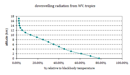
I related this to the blackbody emissions for the respective temperature, at the respective altitude, thereby sorting out an otherwise strong temperature bias. Of course water vapor thins out with altitude and so does its optical thickness. These data still contain a substantial amount of (cumulative) downwelling radiation from the stratosphere above.
Another, probably more consistent way of looking at it, is by comparing upwelling radiation by altitude and again relate it to the blackbody radiation at the respective temperatures. I know, I could spent eternities explaining this “fool proof” to people not so fit cognitively, but just let us assume that was not the issue here, lol.
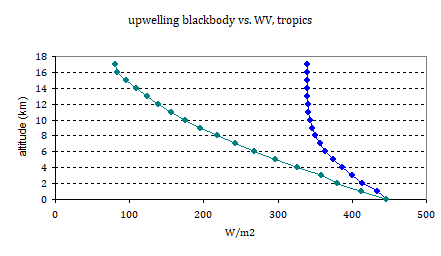
What it means is, the blue line represents the upwelling radiation as given in modtran, for the respective altitude (looking down), with WV only and all other GH-agents removed. The teal line gives the blackbody radiation, based on the SB-law, for the respective temperature at altitude (modtran gives the temperature in a chart). If the atmosphere was totally opaque, the blue line would behave like the teal line. The fact that it does not and barely decreases past 10km altitude, indicates a (very) low optical thickness. Alternatively, if the atmosphere was perfectly transparent, upwelling radiation would not decrease at all with altitude.
Think of it like this. If there was a slab layer at 10km altitude, like an optically thick cloud layer, modtran would not give us 343W/m2 in upwelling radiation (blue) there, but only 175W/m2. Going from 9 to 10km in altitude, upwelling radiation would need to drop by 171W/m2 if there was something perfectly opaque. The actual drop off in the model is just 3.14W/m2, and so we can relate these two figures (3.14/171= ~2%) to determine the relative opacity of the respective layer within the model. Et voila!
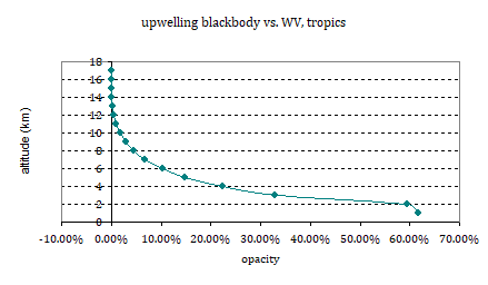
While it is still not perfect, it gives us a very good view on the optical thickness of WV by altitude as represented in the inner tropical scenario in modtran. To provide context, the S05 chart shows about 50% lapse rate effect at ~5.2km altitude, about 100% at ~7km and about 150% at ~10km. In other words, at those altitudes warming considerably more than the surface, thereby potentially holding accordingly more WV and producing more WVF, the optical thickness of WV runs so low, that it barely matters. I mean it does matter, but the impact is limited.
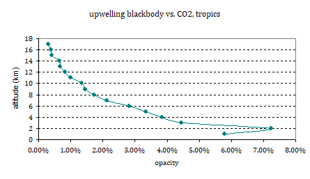
Among the many “background checks” I tend to do, I applied the same procedure on CO2. I know, there is a little issue here with the finite resolution of modtran, yet it beautifully shows how CO2, other than WV, maintains its optical depth relatively well with altitude. Of course, nothing else was to be expected. The reversal at the lowest layer is at least partly due to modtran having different emissivities for surface and GH-agents, btw.
Thus projecting the theoretic(!) lapse rate change (not the lower climate model outputs) point for point onto the respective optical thickness, yields an increment of 35%. I will skip the details of the projection, it is just about weighting the lapse rate effect with the respective share of the individual altitudes in the upwelling radiation. It as close as I can get to the “radiative kernel” approach I can get. It means if modtran did incorporate a changing lapse rate, the clear sky WVF there would not be just 1.727W/m2, but about 2.33W/m2, while the all sky reality it will be around 1.35W/m2. In the outer tropics it should be a similar figure, as the relative scarcity of WV and clouds largely cancel out. And that is that.
Is there a chance modtran is wrong? Yes, because it will generally overstate WV, as discussed before. However, in the given context, this bias could also work in the opposite direction. If the optical thickness is overstated at lower altitudes, then the share of WVF from the lapse rate insensitive emissions would equally be overstated, and the lapse rate effect understated. It would not make much of a difference however. Apart from that issue, I have not even accounted for the stratosphere blocking a small share of the outgoing radiation, thereby also mitigating WVF.
One could also think of it like this. If the OLR emissions profile (by altitude) of WV would equate to the global average of GH-agents, the enhancement of WVF due to the lapse rate effect would equate to the increment of emission temperature relative to the surface temperature, or about 1.8, as discussed above. But because WV is not a “well mixed GHG” evenly distributed over the atmosphere, but instead strongly bound to low altitudes, both in terms of concentration as well as optical thickness, that figure must be undercut by a significant margin. It is the exact opposite with clouds btw.
So we have the model output as in ZH11 assuming some 3.8W/m2 of WVF in the inner tropics, as a central estimate, while modtran, if we squeeze out as much information as possible, tells us it is only about 1.35W/m2. Those figures are worlds apart. I think it is not really necessary to comment on it, I have already discussed what the positive WVF illusion is based on, and how this unphysical nonsense is a conditio sine qua non for the climate agenda. Substituting 3.2 for 1.35 in our ECS formula now yields..
-4.2 / (-6.96 + 1 + 1.35) = 0.91K
Only just doing the necessary corrections on the WV part in the tropics drops the (basic) climate sensitivity there from 6.5K to 0.91K. The tropics that serve as heat engine within climate models, turn from being the main asset into the biggest liability. And that is without even discussing the issues with CO2 forcing, or cloud feedback, and there are plenty of them.
Consolidating WV + LR Feedbacks
Based on physical constraints, the theoretically excpected change in lapse rate and the distribution of effective emission altitudes, as in modtran, I have determined both tropical LR and WV feedbacks. We can tell tropical temperature feedback will be about 6.96W/m2. The magnitude of LRF would then depend on what share of it you attribute to the Planck Response. It should be 3.85W/m2 logically, resulting in an LRF of 3.11W/m2, but one could also assume some lower figure, as in the literature, of say 3.6W/m2, with LRF then being 3.36W/m2.
In terms of climate sensitivity this distinction will not matter, but in terms of the combined WV-LR Feedback we want it singled out. Given tropical WVF is only about 1.35W/m2, negative LRF will dominate it by a huge margin in the -1.8 to -2W/m2 range. I just can not stress enough how intriguing this is. It is a massive negative feedback, and yet “consensus science” claims the exact opposite, a equally massive positive WV-LR feedback of some +2W/m2. Consensus science here is off by a jaw dropping 4W/m2 on tropical WV-LR feedback.
The blunder goes back at least to Raval, Ramanathan 1989 “Observational Determination of the Greenhouse Effect” published in the poor quality, but high impact “Nature” journal. It is hidden behind a paywall, but Ramanathan also discusses all those considerations in this freely accessible and far more recent source11.
Between 10°N and 10°S, dGa/dTs (7–10 W m−2 K−1) exceeds the blackbody-emission value of about 6 W m−2 K−1 , thus reproducing the so-called super greenhouse effect inferred from latitudinal variations in Ga and Ts (Raval and Ramanathan,1989)
We have to bear in mind, however, that both temperature effect (as represented by the Planck and lapse-rate feedbacks) and moisture feedbacks contribute to the observed dGa/dTs
The fundamental issue is about restricting the perspective on those two feedbacks, thereby insisting on these being feedbacks, thus physical reactions to Ts. At no point it was even considered tropospheric temperatures might have some life on their own, so to say, and with regard to the (inner) tropics, also restricted by advection. The high horizontal winds speeds at altitude (jet stream) also mean effective communication of the temperatures over latitudes up there. The whole idea is even more absurd, when you know the GHE is about the troposphere dominating Ts, not the opposite way. And even in the daily cycle we see how surface temperature varies over a large range, as opposed to the air above.
I took the data from said Ramanathan publication and matched it versus the UAH lower troposphere base. Both represent the annual temperature (variation) for tropical latitudes between 30°N and 30°S, thereby also representing 50% of the whole Earth. With the assumed negative LRF the variation in Tlt would need to be larger than that of Ts..
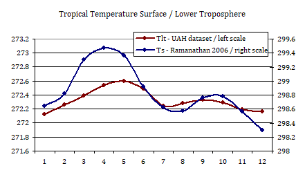
It turned out the annual temperature range (ATR) is 60% lower within the lower troposphere than at the surface. If the data are correct, and as far the lower troposphere represents the effective emission temperature (Tz), this will explain the bulk of the “super GHE” Ramanathan claims, but has nothing to do with the GHE, nor with feedbacks. Instead it is just some healthy autonomy of the troposphere. But it will not matter anyway, because even if one considers this a positive LRF over seasonal variation of Ts, we still know it will be negative with long term global warming, and so it can not serve as the proxy “consensus science” thinks it would.
In the context of “consensus logic” a non feedback, thus Planck Response, would equate to 3.6W/m2 (maybe 3.5, does not matter) in the tropics. If observed dOLR/dTs = 0, it can be condensed into this little restriction...
WVF + LRF - 3.6 = 0
Then assuming LRF has to be negative, like -1W/m2, you will have to conclude the presence of a massive positive WVF, like..
4.6 - 1 - 3.6 = 0
Sure you can reduce WVF somewhat if you assume a somewhat smaller Planck Response of 3.5, or consider clouds playing into it, or when there is a least some dOLR/dTs above 0, meaning a small negative term on the right side in the restriction above. But either way, you would conclude a huge positive WVF term. And that is exactly what we have in Ramanathan’s work, many other publications, and throughout the models.
If however we consider reality, where dTz/dTs might be ~0.4, we will a very different outcome. LRF will become a positive (pseudo-) feedback of ~2.4W/m2 (=260^3*4*5.67e-8*(1-0.4)). Then said restriction will be fulfilled with a much smaller WVF, like..
1.2 + 2.4 – 3.6 = 0
Now other than with the restricted and misleading view on seasonal variation of Ts, we still know that LRF will be negative with actual global warming and that it will be a large term, at least -3W/m2 in the tropics. A combined WVF + LRF term will then show a large negative feedback like 1.2 – 3 = -1.8W/m2. Although one could certainly make a case in arguing WVF would not serve as a reasonable proxy here either. But that should not be much of a problem, given we have already derived a 1.35W/m2 WVF from modtran.
Conclusion
The “super greenhouse effect” in the inner tropics, as well as the very strong GHE all over the tropics as deducted from seasonal variations in temperature, is not real, but an artefact. The inertia of tropospheric temperatures as well as the effective emission temperature (Tz) has been mistaken for a sign an extraordinary strong water vapor feedback. The assumption is dTz/dTs > 1, while actually it is ~0.4. Equally it has been assumed the observed dOLR/dTs relation would include a negative lapse rate feedback, without ever verifying said assumption, in an act of unspeakable hubris.
It is unthinkable this blunder went unnoticed for decades, however I could not identify any critical discussion on the subject. Yes, I seeked the help of AI to identify such discussions, but while it provided me with a lot of sources, they were all dead ends or hallucinations. It seems likely no such considerations have ever been made public. Since it would kill off the climate agenda instantly, there might be strong incentives not to do it, at least within the community.
The initial incentive, discussing the argument over the lapse rate issue being something of the tropics (only), while strongly diluted by opposite lapse rate effects at higher latitudes, has yielded plenty of results. Focusing on the situation in the tropics reveals there is no remedy to be found, but rather the essence of the problem. Approximately WVF has been overstated by ~2W/m2, while LRF has been underestimated equally by about 2W/m2, adding up to a total error margin of ~4W/m2.
Tropical combined WV + LR Feedback is not strongly positive, but instead strongly negative. This also solves the issue over theoretic climate sensitivity, as in climate models, being highest in the tropics, while actual surface sensitivity is definitely at its lowest there. And of course it equally has all the ramifications on global climate sensitivity.
Comments (0)
No comments found!