

A Falsification - the incredibly stupid case of water vapor feedback
In one of the last articles I investigated the “radiative flux” (sic!) concept. With it, although I am afraid it is based on really bad logic, it is at least possible to reproduce the canonical CO2 forcing estimate of some 3.7W/m2. However even this theoretical approach is no remedy for a (primary-) water vapor (WV) feedback of some 1.8W/m2. There is simply no way to get even close to this figure. Even if you push all the limits, you will get no higher than 1.2W/m2. I mean it will be a lot lower anyway, as WV is vastly overrated as a GHG.
The situation is odd enough, given radiative transfer models contradict the common feedback figure. It is nothing you could ignore, at least not in any real science. In “climate science” however nobody seems to care. For me the problem instead was about not understanding “the science”. Understanding will not mean agreeing with it, but rather being able to reproduce it. You just can not reflect on what you do not know.
Reading the “Clouds and Water Vapor” series of articles on SoD1 helped me out, I guess. There was nothing really new to me, but I neglected it so far. There are a lot of stupid concepts in “climate science” and I tend to ignore them, unless I think they would have some relevance within “the science”. In this instance, I just did not have it not on the radar. Just because it made no sense to me does not mean “climate science” would not heavily rely on it. With the whole SoD article series circulating around this one idea and plenty of high level articles given as source, I realised there is more to it.
Ok, just let me explain in plain words what the whole idea is. It is about relating surface temperature (Ts) to outgoing emissions (OLR), that is emissions top of the atmosphere (TOA) as to be observed by a satellite. In short: the relation dOLR/dTs. Both of which will be empirical data and thus a welcome alternation to otherwise often just theoretical frameworks in “climate science”.
A little exploration of the “Planck Feedback”
If for instance the sun should become hotter, it is obvious this would raise the temperature of Earth. Also the physical relation between energy input and the consequent direct temperature change is simple and undisputed physics. The more complicated question is over how much energy is going to leave the “climate system” (sic!) of Earth due to such a change in temperature. There we have the term “Planck Feedback”, which is not a feedback in any way, but is only describing the increase in emissions due to the Stefan-Boltzmann law. Should the observed change in emissions be equal to this “Planck Feedback”, or proportionate if you will, there would be no feedback. If emissions were changing faster, that will be a negative-, should it be slower, that will be a positive feedback.
The “Planck Feedback” is named to be 3.3W/m2 for Earth as whole, and 3.6W/m2 with clear skies only. This relation is well consistent with the typical size of CRE (cloud radiative effect). There is not much explanation on SoD as to where these figures come from, and so naturally there is some discussion, or even protest in the comments below. It would appear no one really had a clue and so let me sort this out first, since I already explained it.
Again, we have this quote from Cess et al 1990 (C90), clarifying the whole thing, or not respectively. It is simply relating surface temperature to emissions TOA. This relation goes against everything that “climate science” is based on. The GHE is about surface emissions NOT going directly into space and instead being largely substituted by emissions from a much colder atmosphere. Equally, assuming black bodies (bb), we would have 390W/m2 in surface emissions, 240W/m2 TOA and a GHE of 390 – 240 = 150W/m2. It is all simple math.
The SB law:
P = T^4 * 5.67e-8
The first derivation hereto:
P' = 4 T^3 * 5.67e-8
For the a surface temperature of 288K we can calculate the „Planck Feedback“
4 * 288^3 * 5.67e-8 = 5.418
Since we know the emission temperature at 240W/m2 equates to 255K black body temperature(as 240 = 255^4 *5.67e-8), the simplified “Planck Feedback” for emissions TOA will be..
4 * 255^3 * 5.67e-8 = 3.76
Assuming a „Planck Feedback“ of only 3.3W/m2 will require a very different temperature..
4 * T^3 * 5.67e-8 = 3.3
T^3 = 3.3 / ( 4 * 5.67e-8)
T = 244.1K
You never heard about these 244.1K in the context of basic “climate science”? Of course you did not, as it does not exist as such, although it is the only possible bb temperature consistent with a “Planck Feedback” of 3.3W/m2. Instead it is based on a formal impossibility. An increase of 1 at 288 means 0.3472%, at 255 instead it is 0.3922%, which is more. By relating the unrelated 288K to the “Planck Feedback” at 255K, you get those 3.3 (= 3.76 * 255 / 288). It is nonsense, period. However, it is nonsense increasing climate sensitivity and so it appears sacrosanct. The author of SoD just does not have the will, or skill, to question such things.
Just if you wonder the C90 quote above is so simplistic, let me help you out. We already know..
288^4 * 5.67e-8 = 390.08
We can enhance the first derivation unnecessarily by dividing it by T (T^4 / T = T^3)
P' = 4*T^3 * 5.67e-8 = 4*T^4 * 5.67e-8 / T
Then the term T^4 * 5.67e-8 is just the plain vanilla SB law. We can substitute with the result we already know..
4 * 390.08 / 288 = 5.418
It is the same result as above. The only thing C90 did was illicitly relate the unrelated figures 288K and 240W/m2..
4 * 240 / 288 = 3.33
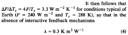
Inverting this erroneous “Plank Feedback” number then gives us λ = 1 / 3.33 = 0.3, with Lambda being for W/m2 (be it forcing or feedback) to temperature. The formula for ECS then basically goes like this (F – Forcing, FB – sum of primary feedbacks)..
ECS = F * λ / (1 – FB * λ)
If we take very typical figures both for F (3.7) and FB (2.1), then ECS would be 3K..
3.7 * 0.3 / (1 – 2.1 * 0.3) = 3
..whereas a more accurate Lambda of 0.27, with otherwise identical forcing and feedbacks, will only yield an ECS of 2.3K
3.7 * 0.27 / (1 – 2.1 * 0.27) = 2.307
In general the Lamda issue overstates climate sensitivity by about 30%. The error margin will be even higher for larger feedbacks. Strangely this follows a simple pattern. With an ECS of 2K it will be 20%, with 3K 30%, with 4K 40% and so on. I discussed the details hereto already.
Anyway, the “Planck Feedback” should be 3.76 for all skies and about 4.1W/m2 with clear skies only. The latter correspond to emissions in 268W/m2 range, which is consistent with an average bb emission temperature of just over 262K. Needless to say it is because we have a larger atmospheric window without clouds, and lower emission altitude within the atmosphere.
On with the show
Sorry for annoying you with these details, but they are an important framework, especially for what is to come. The “Planck Feedback” will serve as the benchmark and observational data should teach us about possible (fast-) atmospheric feedbacks. Fast atmospheric feedbacks? Well, that comes essentially down to water vapor, including lapse rate feedback. Cloud feedback is naturally ruled out if we only look at clear sky scenarios. Equally albedo feedback will not matter.
SoD starts with a contribution from Ramanathan from the book “Frontier of Climate Modelling” by Kiehl, Ramanthan 2006 . Ramanthan is nice to read. He is pretty straight forward and logical (until he is not) with a plain language. He is not into cryptic, ambiguous formulations trying to hide the concept, like many “climate scientists” regrettably do2.
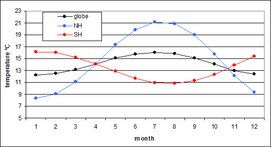
He presents, among others, this amazing chart (Figure 5.10.):
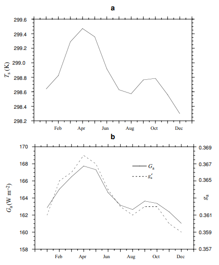
What we have here is the surface temperature (might as well be meteorological 2m temp.) in the tropics (30°S to 30°N). Over the cycle of the year, although there are no outspoken seasons, it shows a little variation. The GHE shows a striking correlation to it. The warmer it is, the more WV in the air, the less radiation goes out into space and the larger the GHE. That is the concept, that is the idea. Obviously this would imply a strong positive feedback. The capital “G” here refers to the GHE in W/m2 as with the left scale, the “g” gives the GHE as a fraction of surface emissions, right scale.
At the first glance this might indeed look impressive. When I looked at it however, I was far less impressed and rather my jaw dropped. I thought, are you serious? That is because I saw something this chart conceals. To explain it I had to extract the data, point for point, which is quite annoying. But with these data, once roughly recovered, we can do some amazing things.
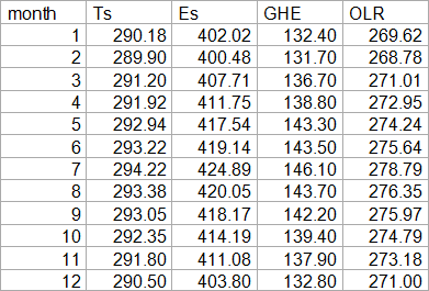
This follows the classical definition of the greenhouse effect, which is the effect of the atmosphere in reducing the longwave cooling to space. The term Ga is defined as Ga = E − Fc where Fc is the measured OLR for clear skies and E is the emission from the surface, which for a black body equals σTs^4 with σ = 5.67 10−8 W m−2 K−4 and Ts is the surface temperature.
From the chart we can only tell surface temperature and the GHE. But the GHE, and this is well defined by Ramanathan (see quote above), is the difference in surface emissions (Es) and OLR. Also he suggests the surface behaving like a bb. It follows we can calculate surface emissions based on surface temperature. And since we then already have two variables of the GHE equation, we can easily calculate the third one.
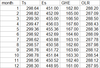
To illustrate the two main variables let me show them in a chart. Although there are two separate scales to move the curves closer, both scales have the same interval.
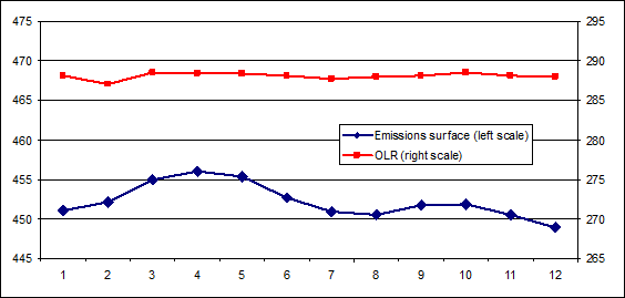
OLR is basically flat, and most of all not showing any correlation to surface temperatures. Sure, you can interpret this in the way “climate science” does. The WV FB is so strong there that it completely cancels out the “Planck Feedback”, and just incidentally we end up with flat OLR. Ramanathan, and the whole of “climate science” with it, names this:
“enhanced trapping in the equatorial regions”
..and even suggests a “super GHE” in the inner tropics:
“Between 10◦ N and 10◦ S (not shown), dGa/dTs (7–10 W m−2 K−1) exceeds the black body-emission value of about 6Wm−2 K−1, thus reproducing the so-called super green house effect inferred from latitudinal variations in Ga and Ts”
The term “super GHE” is a bit misleading. Basically he means a primary feedback above 1. I have already discussed how this is a logical impossibility in general, because then the climate of Earth (or any system) would want to tip over in one or another direction at the slightest perturbation. To a forcing of for instance 1K you get a primary feedback of 1K (or higher), which triggers another feedback of 1K (or higher) and so on. Indefinite warming and a runaway GHE were the consequence. Ramanthan was certainly aware of this implausibility. He only suggests this to be true for the inner tropics and any such tendencies of a runaway GHE there, would be held back by the global climate “system”, where the feedback response would be much lower.
Anyway, the flat lined OLR deserved a lot more attention, rather than being hidden away. You do not want to assume malice, but it is quite obvious how this detail alone can easily destroy the whole argument Ramanathan is trying to make, and the basic narrative of “climate science” with it. What if atmospheric temperatures (Ta), from where most of the emissions TOA occur, are simply not well correlated with surface temperature and OLR therefore not related to Ts? You know there is this famous saying correlation does not necessarily mean causation, and it is true. But here we have the problem inverted. If there is NO correlation, why would you take causation for granted? It is a bit absurd.
Ramanathan provides another example, this time for the whole of Earth, except the poles. That is probably why average temperature here is about 4-5K warmer than the actual global average.
In this instance OLR is at least not perfectly flat. This would make it a bit more plausible that we are not looking at something else, but that it could actually reflect WV feedback. Yet there is a problem. We already know this ~4K temperature variation over the year is not due to the tropics, where temperatures barely change at all and definitely do not peak in July. Instead this is entirely caused by NH land masses above 30°N, that have no counter part in the oceanic SH. In some parts of Siberia the average temperature in July is about 60K higher than in January. With the Falkland Islands for instance, a high latitude SH location, this spread is only 9K, or only 6-7K with South Georgia or the Kerguelen Islands. As in the chart below, the global temperature variation is due to the NH variation dominating the much smaller one in the SH.
It is also worth noting that over the cold winter the plains of Asia, North America and to a lesser degree Europe, will feature strong inversions. At the same time there are large atmospheric windows. Under these circumstances those plains radiate their extreme cold directly into space so to say. It is not so much the warm summers increasing emissions TOA, but rather the cold winters reducing them, if that makes sense. It is NOT due to the sun btw., which is about 7% stronger in early January than in early July and thus acts counter-cyclical. If it was the sun and surface was adapting fast enough (it is not!), global temperatures could be over 4K higher in January than in July.
If we simplistically assume a clear sky atmospheric window of about 30%, and it will be substantially larger over mid to high northern latitude land masses, we can explain the variation in outgoing emissions almost entirely. The term becomes minimal with a 37% window btw.
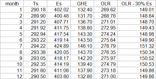
Again it seems outgoing emissions are barely related to surface temperature, except for the atmospheric window. As before, it is ambiguous information. Either WV is almost perfectly compensating the variation in surface temperature and thus is a huge feedback, bigger even than what “climate science” assumes, thereby suggesting ECS would thus be even larger, or there is simply some misunderstanding.
Of course there are a lot more papers dealing with this kind of research. They all more or less come up with the conclusion already named in R06:
“Radiative-convective models with fixed relative humidity assumption yield (e.g., see Ramanathan et al., 1981) dFc/dTs ≈ 2Wm−2 K−1.”
The same conclusion is drawn in the SoD article number 93, doing some proper genuine research there. The idea and the results are highly consistent. Emissions TOA fall far short of the “Planck Feedback”, indicating a positive feedback with clear skies. It is about 2W/m2 instead of the 3.6W/m2 expected.
The Relation dGHE to dOLR
The GHE on the other side is expected to grow and shrink along with variations in surface temperature anyway. We recall surface emissions would grow by 5.4W/m2 for every Kelvin in dT. Accordingly, if the GHE grew only 1.8W/m2 (5.4-3.6), this would indicate a non feedback response. I can smell the odor of confusion! The reason is that even if there was a symmetric increase in temperature throughout the surface/troposphere “system”, emissions are a function of temperature by the power of 4. So if the surface warms by 1K AND the troposphere warms equally by 1K, though at a lower absolute temperature, emissions TOA will grow by less than surface emissions. How much exactly it would grow, that will depend on the discussed assumptions.
Anyway, within the given logic a dGHE of above 1.8W/m2 would indicate a positive feedback and so will a dOLR of less than 3.6W/m2. Equally a dGHE of 5.4W/m2, or dOLR of 0, would indicate a perfect, total feedback so to say. So it is 1.8 – 5.4 with dGHE and 3.6 to 0 with dOLR for zero to maximum feedback. It is the same thing, just with different scales and different signs. The above 2W/m2 figure will then translate into dGHE of 3.4W/m2 (= 2 - 5.4).
Some empiric climate data
To understand the fundamental problem, let me show some basic climate data from four arbitrary locations in and around Austria4. There is nothing special, just the ordinary data climate data you would typically find on wikipedia if you looked up a certain place.

(to the left in “dT” there is the annual temperature range (ATR) on top, and daily temperature range (DTR) on the bottom)
Both Zell and Spittal are smaller alpine towns with a typical climate for this region. The Sonnblick however is a bit special as it represents an old weather station located on a mountain top at 3,100m altitude. It is roughly between the two named small towns. I have also added the “Zugspitze”, which is the tallest mountain of Germany (2962m), but actually at the border between Austria / Germany, and is roughly 100 miles to the west relative to the other three locations.
Nominally these are all surface stations, yet there is a huge difference between those in the valley (or lowlands) and those on mountain tops. Air will typically move heat horizontally, why it is also called advection rather than convection in meteorology. A mountain top is thus like a probe within the atmosphere at the respective altitude. There will be some micro mountain climate so to say, but largely it will represent the atmospheric temperature there. Sure there are “cleaner” ways to measure atmospheric temperatures, but they all have their issues. Weather balloons or aircraft can give you sample data, but they can not hold a certain position and give you consistent data. Ideally we would build towers reaching kilometers into the sky, but that is beyond our means. When it comes to consistent data from within the troposphere, mountains are as good as it gets.
The daily temperature range (DTR) is one thing that distinguishes such mountain climate. To some it may come as a surprise, but the DTR is a lot smaller. There is this myth, spread by NASA5 among others, that GHGs were restricting the DTR. The dry air over the Sahara would then explain a huge DTR to be observed there. Both is wrong of course. Neither is the DTR specifically large in the desert, nor is WV (or the lack of) the cause for it. Equally GHG concentration over such mountain tops is pretty low, but that has no impact on DTR.
The whole atmosphere has a mass equivalent to 10 meters of water, while it receives only 1/3 of the absorbed solar radiation. The surface on the other side is a relatively shallow layer (talking about land, not water) receiving 2/3s. Unsurprisingly the solid surface heats quickly in the sun, while the troposphere behaves sluggish. The same goes for the cooling process. It is even more extreme if we talk actual surface temperature, and not just meteorological 2m temperature. That is also the mystery behind the “unusually large DTR” in the desert btw.
Also the WV amount remains pretty stable over the day/night cycle, with only relative humidity changing due to temperature variation. For these reasons it makes no sense to compare DTR variation of the surface to OLR. You would find that emissions, coming mainly from the sluggish troposphere, barely react to changes in surface temperature, far less than the “Planck Feedback”. You might then conclude the presence of strong WV feedback and very high ECS, but it would evidently all be wrong. “Climate scientists” are aware of the problem and so nobody, thank god, is making this mistake. I mean, not exactly this mistake.
With regard to seasonal cycles it is a different story. Theoretically, over the course of the year, the troposphere should have enough time to adept to solar intensity. Surface- and tropospheric temperature should then move in parallel, and if not, that would be caused by a change in the lapse rate due to WV and the latent heat it transports. This is equivalent to the lapse rate feedback (LRF) and so intra-annual variations in surface temperature should provide a perfect opportunity to investigate VW feedback, although it would not distinguish between WV feedback in the narrow sense and LRF.
The only problem is, as the climate data above reveal, it does not work a single bit. The same issue that invalidates DTR variations for this purpose also applies for annual temperature range (ATR), just for a different reason. In the named two towns the ATR is 22.6K and 20.6K respectively, quite typical for the region, while on the two mountains it is 14.5K and 13.6K, roughly a third less. Notably the lapse rate should decrease with warmer and increase with lower temperatures (just check for wet and dry adiabat). If that mechanism was in play, the ATR should be larger on mountain tops, not smaller.
What happens for real is convection, or in terms of meteorology, mainly advection. The horizontal transport of heat is far more effective within the middle to higher troposphere, than it is towards the surface. The wind speeds are high, the heat loss relative to the heat capacity is small, while with the surface it is the opposite. It is also the reason for the typical winter time inversions we see in higher latitudes. In fact such inversions themselves are well documenting the basic issue. Over the seasonal cycle surface (or close to surface) temperatures are way more variable than tropospheric temperatures. But it is this troposphere which is responsible for the bulk of outgoing emissions.
So of course OLR shows far less variance than the surface temperature, but that is because the troposphere has a smaller ATR. It has NOTHING to do with WV feedback. It is like watching clouds and seeing a face. That is because we are naturally inclined to identify faces, not because there was one. We tend to see what we want to see. In this instance “climate scientists” wanted to see indications of a strong WV feedback
UAH temperature data
But there is yet more evidence. The question is on tropospheric temperature records, as opposed to surface temperature. Where could you possibly find these? As so many times before it was an iterative process to get what I needed. The UAH data set has four different flavours (low-, mid troposphere, tropopause, lower stratosphere) and only gets published as a deviation from average. But I was interested in the low- to mid troposphere temperature variation within the annual cycle, rather than any departure from normal. The “normal” was the subject of interest.
After some research and communication I found the “tltmonacg_6.0”6 file on the server contained all the “normal” values7. There are some issues with these data after all. It turned out the lower troposphere temperature, and that is the one we are most interested in, is actually not measured but rather invoked from the other results, with the scheme..
TLT = 1.538*TMT – 0.548*TTP + 0.10*TLS
..if that is true. Feel free to join the discussion in this subject matter8. While this may cast some doubt on the UAH temperature record as such, we are not here to do that. I am quite aware this temperature record is not so beloved by “consensus science” just because it produces less warming than some other records. If however there was a fundamental issue with the baseline, I would assume it had been tackled a while ago. Also the UAH record does not diverge a lot from the RSS global temperature (also satellite) record.
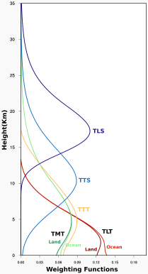
Then of course the microwave remote sensing is complicated and can not give the exact temperature at a certain altitude. Rather it is about an altitude range (as in the chart above)9. For instance the average temperature given for the lower troposphere is around 263K, that is at least 25K colder than the actual surface. Bear in mind the UAH data exclude the 7.5° of the highest latitudes at the poles, meaning a warm bias. The “lower troposphere” thus is not that low, in fact it will be at least 4km up in altitude. Anyway..
I took the average surface temperature from climatereanalyzer.org10 and plot it against the averages from UAH for both the lower and the mid troposphere11. The result is shown in the chart below.
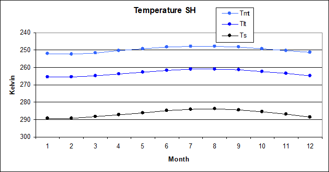
As with the SH the result is nothing spectacular. The ATR is 5.3K with the surface, 4.6K with the lower troposphere and 4.4K with the mid troposphere. When relating dOLR to dTs this somewhat smaller ATR up the atmosphere is certainly something you will have to consider.
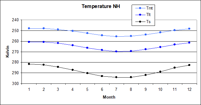
With the NH, as to be expected, it is a different story. Here the ATR is 12.8K with the surface, 8.9K with the lower- and 7.6K with the mid troposphere. Although within the troposphere the ATR is still a lot larger than in the SH, it just can not keep up with the large ATR over NH land masses. Here it would already be a fatal mistake to ignore sluggish tropospheric temperatures when looking at the dOLR/dTs relation. Practically, again under consideration of the atmospheric window, the “Planck Feedback” should be undercut by about 25% just because of it, and NOT because any WV feedback.
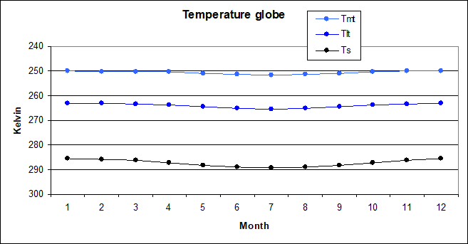
The global scale however is where the problem becomes most pronounced. Because ATRs are relatively small in this instance, it may not be well visible in the chart. Surface ATR here is merely 3.8K, but it shrinks further to only 2.24K with the LT and just 1.7K with the MT. That is 41% and 55% less respectively.
Recursive Quality Assurance
Let us contrast these findings the common understanding as represented by Chung et al 201012
“under the idealized assumption of a horizontally and vertically uniform temperature change, the global-mean clear-sky OLR should increase by 3.6 W m−2 for every 1-K increase in surface temperature.”
“we demonstrate a strong covariance between temperature and water vapor that is robust across all models, is quantitatively consistent with satellite observations”
“The observed rates of radiative damping from regional, seasonal, and interannual variations are substantially smaller than the rate of Planck radiative damping (3.6 W m−2 K−1), yet slightly larger than that anticipated from a uniform warming, constant-RH response (2.0 W m−2 K−1). Such difference could be attributable to either variations in relative humidity and/or departures from non-uniform warming. To better evaluate the implications of such metrics, it is useful to directly compare the observed rates of radiative damping to those obtained from climate models subjected to the same analysis.”
“good agreement between satellite observations and model simulation confirms the robustness of positive water vapor feedback”
The message is pretty clear I guess. You have observations on the one side, models on the other side and they both fit very nicely. For anyone with a brain cell that would confirm both the physical understanding AND model integrity. For those with an actual functioning brain however, there might be a certain problem. The models are based on observational data, and their interpretation. Confirming that interpretation by checking back with models, is recursive. It is like writing a text, then copying it and eventually comparing the copy to the original, just to make sure original is flawless. The only thing such “quality assurance” checks is the copying process itself, nothing else.
The wrong interpretation
The interpretation is that any warming would cause a) an increase in WV within the troposphere, due to fixed relative humidity, and b) a decrease in the lapse rate. The latter means the higher troposphere should warm more than the surface, thereby increasing emissions. That is the negative lapse rate feedback. The LRF would pull the dOLR/dTs relation above the “Planck Feedback”, while the damping by WV would eventually push it down to some said 2W/m2, or so. Accordingly the WV feedback itself must be very strong.
This might be a perfectly reasonable assumption, apart from the 2W/m2 figure, in the long run. In the short to medium term however, we know that is not what happens. The relation of delta troposphere temperature to delta surface temperature (dTa/dTs) is not larger, but a lot a smaller than one. This alone already reduces the dOLR/dTs relation well below the “Planck Feedback”. It has obviously nothing to do with LRF, or latent heat. The lapse rate behaves so that it imitates a strong positive feedback, if that is what you are looking for.
Like in Platon’s Allegory of the cave “climate science” interpreted something into the shadow of dOLR/dTs that fits its beliefs, but stands in stark contrast to reality. The blunder could easily have been avoided and resolved by checking atmospheric temperatures, rather than relying only on assumptions. It seems that never happened. And as far as it did, it invalidated the procedure. More on that later.
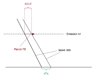
As a chart the logic would look like below. An increase in surface temperature would go along with a slight rotation of the lapse rate. This rotation, or the LRF, would push dOLR beyond the “Planck FB”. As dOLR is far smaller than the “Planck FB”, this would indirectly prove the presence of WV FB raising the emission level higher up the atmosphere, where it is colder and emissions thus smaller.
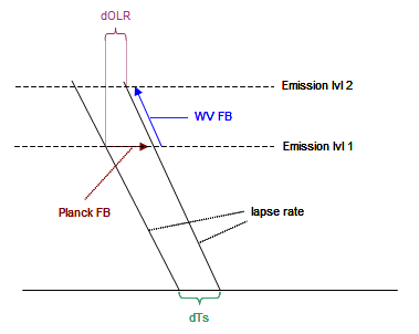
In reality the lapse rate rotates in the opposite direction. This alone suffices to explain how dOLR undercuts the “Planck FB”. There will likely be a WV FB in play on top of that, but it will be a lot smaller and impossible, or at least very hard to quantify. LRF might also exist, but its signal will be impossible to detect. Any attempt to derive WV feedback from the dOLR/dTs relation will be futile.
The Confirmation Bias
Of course the dOLR/dTs analysis comes in different flavors. We could imagine at least five different approaches that all require a change in surface temperature.
- a) Daily temperature variation.
- b) Seasonal temperature variation
- c) Interannual temperature variation (like ENSO)
- d) Regional variations - that is basically climate by latitude
- e) Long term climate change, as with current “global warming”
- f) Radiative transfer models
Option a) would not yield any reasonable result and is not being used. Option e) would be the most accurate one, as over the course of 10, 20 or more years, you could definitely expect Ta and WV to have adapted to increasing Ts. The problems then are of technical nature. You would need to have very well calibrated instruments to make data perfectly comparable over decadal periods. On top of that there will issues with declining relative humidity and so on. To my knowledge it has not been tried anyway.
Even if, it would probably be in vain. To quote AR5: "There is some observational evidence (Section 2.4.4) suggesting tropical lapse rates might have increased in recent decades in a way not simulated by models". Ouch! If that is so, we have no clue what is going on. The lapse rate should be shrinking with growing temperatures. And please see the irony. The whole claim of a positive WV feedback is founded on the notion of perfectly understanding what the lapse rate will do.
That leaves us with options b) to d), which in the literature tend to give relatively consistent results. This consistency is then reinsured by comparing them with model outputs. The impression certainly has to be that the “gold standard” is being applied. You look at a question from multiple perspectives and they all align nicely. Not that you could ever achieve positive certainty in science in the sense of proving something. Certainty is rather achieved by falsification. But as far as attaining a maximum level of confidence goes, this is as good as it gets.
Yet it all falls apart once we take a closer and critical look. I already pointed how checking back with models is recursive und thus worthless. Options b) and c) both suffer from the fatal mistake thoroughly explored here. Not just will these approaches not give us any valid information on real WV feedback, but we also understand how gross negligence introduced a fatal mistake making “climate scientists” believe in the existence of positive WV feedback in the first place.
Option f) is easily available and could have been used to gain confidence. As discussed however, such data contradict the consensus position and thus have been ignored. This fact alone is appalling. And so the only “pillar” left is option d), which on its own, given opposing results from other sources, has no relevance anyway. The “regional” approach suffers badly from being static and having Ta dominated by convective processes. By and large the lapse rate increases with Ts, which is why we have inversions in high latitude winter. This is the exact opposite of what is to be expected in the course of climatic changes. Dessler et al 200813 (D08) thus concludes..
This is a quantitative estimate of the effect of the changing lapse rate on dOLR/dTs, and it shows that it is negative for almost all values of Ts. In other words, as Ts increases, so does the lapse rate, and the general effect of this is to reduce dOLR/dTs, and therefore OLR, below what they would be if the atmosphere maintained a constant lapse rate.
In most climate-change scenarios, the upper troposphere is expected to warm more than the surface, and the additional radiation from a warmer upper troposphere will act as a negative feedback on the warming.
This result demonstrates the unsuitability of using variations in different regions in our present climate as a proxy for climate change.
Yep! Option d) was pointless from the start and should never have been used to provide false certainty. It is also worth noting D08 actually takes Ta into account, something that could easily have avoided the blunders we are discussing. So the incredible is true. All the different perspectives seemingly adding up, are all corrupt, without exception. Not a single one actually makes the slightest sense. They were all driven by incredibly stupid mistakes, or malice. And as far as evidence clearly pointed towards the inconsistency, it was simply neglected. Confirmation bias at its climax!
The claim of a (strongly) positive WV feedback is based on nothing. It makes it somewhat understandable how the canonical 1.8W/m2 figure, plus/minus whatsoever, has remained untackled for so long, unlike the magnitude of CO2 forcing for instance. You can not possibly improve it, but only break it. As it plays such a crucial role in the “global warming” narrative, it must have been sacrosanct.
Let me note two more points, which some people consider a remedy after all. Sure there will be a lot more literature on this subject out there and I have no intent to read them all. There might be variations in the logic, other data sources and so on. What I am discussing here is not a formal, but a material mistake with huge error margin making the “result” point in the wrong direction. It is a definite falsification of the basic concept. You can not “fix” that with a cosmetic rework, a 2.0 version of the same stuff. Also science must not be result driven.
The other point is on how WV concentration reacts to Ts. I neglected this question for good reasons. One might reasonably assume WV to be rather related to Ta than Ts, while in the literature Ta is being ignored in the first place. Then we would need to discuss what is actual data and what are rather model assumptions. Most of all however, we already know the theoretic pathway delta WV -> delta OLR based on radiative transfer models is not working. It gives completely different, much lower results.
Summary
Ok, it was a long story, but one needs to honor the magnitude of the finding. “Climate science” tried to identify WV feedback based on a theoretical framework that consists of an (erroneous) “Planck Feedback” and the idea any deviation from it could only be due to the components of WV feedback (radiative- and lapse rate-). Furthermore there is the assumption tropospheric temperature, over the course of the seasons, or interannual variations, would have enough time to perfectly synchronize with surface temperature according to the above framework.
Given the global average temperature variation is dominated by the specific topography of NH land masses, or ENSO events in the case of interannual variations, and NOT by the heat content of the whole system, the whole idea seems quite naïve. Indeed tropospheric temperatures are relatively autonomous compared to changes in Ts. The lapse rate thus is positively, not negatively correlated to Ts. This “detail” is responsible for the bulk of the observed departure from the so called “Planck Feedback”, not WV feedback.
So yes, the concept of a strong, positive water vapor feedback is based on an amazingly stupid mistake, nothing else. And of course all the books on “climate science” need to be rewritten.
7To read it you will have to apply a 144x72 grid cell, each representing 2.5° of the globe (as opposed to 360x180), with the most 3 northern and southern latitudes not providing any data, cause satellites. The data go from south to north and from Jan to Dec. Every single grid point consumes 5 bytes with temperature in Kelvin, like "24668" = 246.68K.
Comments (1)
LOL@Klimate Katastrophe Kooks
at 02.05.2024That's why water acts as a literal *refrigerant* (in the strict "refrigeration cycle" sense) below the tropopause.
The refrigeration cycle (Earth) [AC system]:
A liquid evaporates at the heat source (the surface) [in the evaporator], it is transported (convected) [via an AC compressor], it gives up its energy to the heat sink and undergoes phase change (emits radiation in the upper atmosphere, the majority of which is upwelling owing to the mean free path length / altitude / air density relation) [in the condenser], it is transported (falls as rain or snow) [via that AC compressor], and the cycle repeats.
Think of the planet's surface as analogous to the evaporator section of a world-sized AC unit, and you come closer to reality than any climate models ever could or can. Space is then analogous to the AC condenser; polyatomics are then analogous to the working fluid, their DOF determining to what extent they contribute to surface cooling, and homonuclear diatomic and monoatomics are then analogous to noncondensable gases in an AC unit (they dilute the coolant gases and thus reduce the efficiency at which energy is transited from evaporator (ie: the surface) to condenser (ie: space).
Under this more-realistic paradigm, polyatomics are net atmospheric radiative coolants; and monoatomics (and to a lesser extent, homonuclear diatomics) are the actual "greenhouse gases".
This is why water vapor reduces the Kelvin-Helmholtz Gravitational Auto-Compression Effect (aka the lapse rate)... it increases thermodynamic coupling between heat source (the surface) and heat sink (space). It convectively attempts to reduce temperature differential with altitude (ie: reduce the lapse rate) at the same time that it radiatively emits higher in the atmosphere at a faster rate then it can convectively warm that same emission height.
Think about it this way... we all know the air warms up during the daytime as the planet's surface absorbs energy from the sun. Conduction of that energy when air contacts the planet’s surface is the major reason air warms up.
How does that ~99% of the atmosphere (N2, O2, Ar) cool down? It cannot effectively radiatively emit.
Convection moves energy around in the atmosphere, but it cannot shed energy to space. Conduction depends upon thermal contact with other matter and since space is essentially a vacuum, conduction cannot shed energy to space… this leaves only radiative emission. The only way our planet can shed energy is via radiative emission to space. Fully ~76.2% of all surface energy is removed via convection, advection and evaporation. The surface only radiatively emits ~23.8% of all surface energy to space. That ~76.2% must be emitted to space by the atmosphere.
Thus, common sense dictates that the thermal energy of the constituents of the atmosphere which cannot effectively radiatively emit (N2, O2, Ar) must be transferred to the so-called ‘greenhouse gases’ (CO2 being a lesser contributor below the tropopause and the largest contributor above the tropopause, water vapor being the main contributor below the tropopause) which can radiatively emit and thus shed that energy to space. Peer-reviewed studies corroborating this are referenced in the attached file.
So, far from being ‘greenhouse gases’ which ‘trap heat’ in the atmosphere, those polyatomic radiative gases actually shed energy from the atmosphere to space. They are net atmospheric radiative coolants.
You will note the dry adiabatic lapse rate (~9.81 K km-1) is due primarily to the monoatomics (Ar) and homonuclear diatomics (N2, O2)... we've removed in this case the predominant polyatomic which reduces lapse rate (H2O)
Monoatomics (Ar) have no vibrational mode quantum states, and thus cannot emit (nor absorb) IR. Homonuclear diatomics (N2, O2) have no net electric dipole and thus cannot emit (nor absorb) IR unless that net-zero electric dipole is perturbed via collision.
In an atmosphere consisting of solely monoatomics and homonuclear diatomics (ie: no polyatomic radiative molecules), the atoms / molecules could pick up energy via conduction by contacting the surface, just as the polyatomics do; they could convect just as the polyatomics do… but once in the upper atmosphere, they could not as effectively radiatively emit that energy, the upper atmosphere would warm, lending less buoyancy to convecting air, thus hindering convection… and that’s how an actual greenhouse works, by hindering convection.
For homonuclear diatomics, there would be some collisional perturbation and thus some emission in the atmosphere, but by and large the atmosphere could not effectively emit (especially at higher altitudes, because the chance of collision decreases exponentially with altitude).
Thus the surface would have to radiatively emit that ~76.2% of all surface energy which is currently removed from the surface via convection and evaporation… and a higher radiant exitance implies a higher surface temperature. The lapse rate would ensure that with a warmer upper atmosphere, the surface would also warm.
The CAGW (Catastrophic Anthropogenic Global Warming, due to CO2) hypothesis has been disproved... it does not reflect reality. It's been disproved via multiple avenues at the link below.
https://www.patriotaction.us/showthread.php?tid=2711
The takeaways:
1) The climatologists have conflated their purported "greenhouse effect" with the Kelvin-Helmholtz Gravitational Auto-Compression Effect (aka the lapse rate).
2) The climatologists claim the causative agent for their purported "greenhouse effect" to be "backradiation".
3) The Kelvin-Helmholtz Gravitational Auto-Compression Effect's causative agent is, of course, gravity.
4) "Backradiation" is physically impossible because energy cannot spontaneously flow up an energy density gradient.
5) The climatologists misuse the Stefan-Boltzmann (S-B) equation, using the idealized blackbody form of the equation upon graybody objects, which manufactures out of thin air their purported "backradiation". It is only a mathematical artifact due to that aforementioned misuse of the S-B equation. It does not and cannot actually exist. Its existence would imply rampant violations of the fundamental physical laws.
6) Polyatomic molecules are net atmospheric radiative coolants, not "global warming" gases. Far from the 'global warming gas' claimed by the climatologists, water acts as a literal refrigerant (in the strict 'refrigeration cycle' sense) below the tropopause. CO2 is the most prevalent atmospheric radiative coolant above the tropopause and the second-most prevalent (behind water vapor) below the tropopause.