

Seeing through the Atmospheric Window
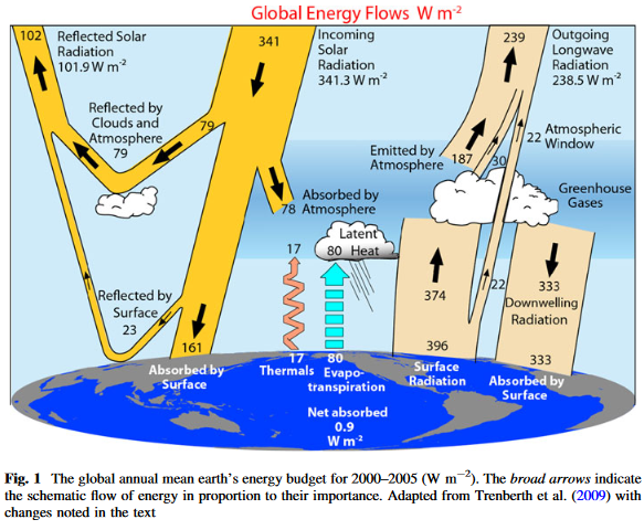
Ok, this is a little issue I ran into and I really wanted to source it out, rather than having it bloating up another article, while not properly addressing it. If you look up the literature, like the famous Kiehl, Trenberth papers, or Wikipedia, you will get a straight forward answer. The atmospheric window is about 40W/m2 in size, and of course it is all settled science.
In reality the settled rather means consensus, and consensus means the abolishment of all scientific principles like pluralism and criticism to promote an all too important message. Just digging a little deeper reveals, as so many times before, huge uncertainty. Ironically it was Trenberth1 himself (with Fassulo, but without Kiehl – T11) who published a totally different version in 2011. There the atmospheric window was almost halved to only 22W/m2. Such an adjustment by a factor of two is not a joke.
Incidentally I also stumbled over Dessler et al 20082, “An analysis of the dependence of clear-sky top-of-atmosphere outgoing longwave radiation on atmospheric temperature and water vapour” (D08). There Fig 8 suggests some 1.25W/m2 increase in emissions TOA for a 1K Ts increase at 288K, due to surface emissions through the atmospheric window alone. This is equivalent to a clear sky atmospheric window of 23% of surface emissions (= 1.25 / 5.4), or about 90W/m2. Also notable:
We are therefore now in a position to explain the evolution of OLR as Ts increases from 273 K to 305 K. The increase in OLR in the midlatitudes, from Ts= 275 K to Ts=290 K, is 32.4 W/m2. Integrating the curves in Figures 8a and 8b, we calculate that increase in Ts directly contributes 22 W/m2, while the warming of Ta contributes 20 W/m2. The increase in q decreases OLR by 10 W/m2.
This suggests a clear sky atmospheric window of 28% = 22 / 76.8 ( = (290^4 – 275^4)*5.67e-8) relative to surface emissions, or roughly 100W/m2 on average over said mid latitudes.
I know, the T11 figure is with all skies, while D08 refers to clear skies. Yet these figures are just way too far apart. Me on the other side, I always had the suspicion the AW should actually be larger than just 40W/m2 and so it all became quite confusing. Either there was something I just did not understand, or something was cheesy. Time to find out!
First I consulted modtran, this time the web app from spectral sciences. Regrettably it is bugged and you can only use the mid latitude summer scenario. Yet this is not much of a problem, as the AW itself is insensitive to most parameters. The lapse rate will not matter, non condensing GHGs do not depend on a certain scenario, and the only thing it comes down to is the concentration of water vapor, and this parameter we can modulate anyway. Just think of the atmosphere as a single layer in this context and the only question being how opaque it is to surface IR (very unlike the GHE itself!).
The great benefit of this modtran version is that we can change the surface temperature, and the surface temperature alone. And although it can not be set to zero, we can set it to 1K, which introduces only a negligible margin or error. We can then compare OLR for a fully radiating surface vs. a non radiating surface and should so identify the size of the AW. Again, this is only for clear skies.
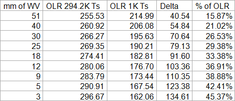
WV is very unevenly distributed over the globe. We have a lot of it in the inner tropics and ~51mm of precipitable water is actually the preset for this scenario, but it can reach up to 60mm. In the dry outer tropics this figure is about 15 to 30mm. In higher latitudes it is strongly depending on the season and the prevailing temperature. Modtran scenarios for mid latitudes reach from 10mm (winter) to 35mm (summer) and 5mm (winter) to 25mm (summer) for sub-arctic regions. In polar regions it may be as low as 3mm. The global average is around 25mm, but a good share of it is concentrated in the inner tropics, where it has “diminishing returns”, so to say.
The weighted global average for the AW should thus be in the 30 to 33% range. With clear skies average OLR is ~270W/m2 (not 240W/m2!), so that we end up with an AWclr of 80-90W/m2. That is well in line with the figures in D08, but above the canonical 40W/m2, and in total opposition to T11.
The implicit question here is about the impact of clouds. First I thought using the (net) cloud radiative effect of some 30W/m2 as the difference between clear and all sky, but that is nonsense. How much surface radiation clouds absorb and their cloud radiative effect are two different things. So, by how much would clouds reduce the AW? The 22W/m2 figure from T11 was adopted from another paper, Costa, Shine 2011 (CS11)3. The paper otherwise does not offer too much innovation, but beautifully outlines the issues there were around before, adding some more to it. With reference to KT97:
The estimate was based on their calculation of the clear-sky OLR in the 8–12-µm wavelength region of 99 W m-2 and an assumption that no such radiation can directly exit the atmosphere from the surface when clouds are present. Taking the observed global-mean cloudiness to be 62%, their value of 40 W m22 follows from rounding 99 x (1 - 0.62).
and..
The effect of clouds is to reduce the STI from its clear-sky value of 66 W m-2 by two-thirds to a value of about 22 W m-2
Again, since Ternberth endorsed this paper by taking on the 22W/m2 figure, we must assume their description of KT97 is correct. If that is so, the theoretical size of the clear sky AW was simply reduced by an equally theoretical cloud fraction of some 2/3s, plus/minus whatever. And that is a big problem.
While indeed there is an abundance of literature pointing out a cloud coverage of this magnitude, it obviously lacks context, which is a problem on its own right. The paper itself names Rossow and Schiffer 19994 with a 67% figure, King et al 20135 would be another source with again 67%. But what does this figure mean? If you looked up into the sky and were to tell what percentage was covered with clouds, that would be a hard question, unless it is completely overcast. It is not just because it was a matter of perspective, or your geometrical intelligence, but also a matter of definition. What is a cloud? The sky may seem clear, but actually be totally covered by subvisual cirrus clouds, which are by definition not identifiable as clouds. The answer might be 0, or a 100%. Good luck with that!
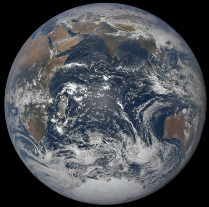
Both KT97 and CS11 assume no surface radiation could go into space in the presence of clouds, so that any cloud was a 100% opaque to LWIR. With regard to optical thickness there is probably not much difference between LWIR and short wave radiation. You only need to look at a satellite picture of Earth6, to understand how most of the surface shines through the clouds, not just a minor share.
But there is more to it. We know clouds have a high albedo. It may be only 50% or less with ice clouds, but water clouds yield 70% and more. Even if we only assume an average 60% albedo and clouds covered like 66% of Earth, the total cloud albedo would amount to 40%, or 137W/m2. That is opposed to some 45 to 50W/m2 cloud albedo effect otherwise named in the literature. These figures are worlds apart. I guess it is easy to see that 67% “cloud cover” does not mean much and is at best to be read as “covered by some clouds”. You may also want to consider the finite resolution, like 1x1° grids, such satellite data have.
Cloud coverage is NOT a binary thing. It is not either overcast or totally clear. Typically we have partial cloud coverage and on top of that, especially thanks to aviation, we have an abundance of thin cirrus clouds with low optical depth. Assuming there could be no surface radiation going into space in the presence of some clouds, is like saying there could be no sunshine unless the sky is perfectly clear. Realistically, considering optical depth, clouds may effectively cover up to 1/3 of Earth, not more. I wish I had a more precise, or official figure here, but we can roughly infer it from albedo aspect anyway. So KT97 should have had an AW no lower than 66W/m2 (= 99 * 0.67) and CS11 no lower than 44W/m2 (=66*0.67). Taking a ~2/3 of cloud cover at face value here is a really naïve and stupid mistake, and not the first of its kind with Trenberth and colleagues.
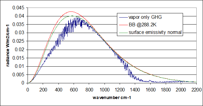
That is if that was the only problem. The origin of the original 99W/m2 seems to be amazingly simplistic. We all know by now (hopefully) that a black body at 288K will emit 390.1W/m2. If you integrate the Planck formula for the interval 8 to 12µm, this segment of the spectrum accounts for 25.3% of total emissions, or 98.7W/m2 (= 390.1 * 0.253). It is easy to see how the 99W/m2 was derived. As in the chart below however, the spectral range of the AW is rather reaching from ~8 to ~13µm, spanning over ~120W/m2 of “black body surface emissions” @288K.
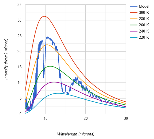
In between we have the absorption by ozone, some weak interference by WV and of course the flanks of the AW can not precisely be defined by a definite wavelength. So 99W/m2, or for the more daring people, a 100W/m2 might be a reasonable guess so far anyway. It is just fascinating of what trivial fabric “state of the art climate science” presented in every text book, as with this instance, is made of. It is pretty wild guessing with a lot of undue simplifications.
And there is yet a deeper problem I have already discussed here, and it is well reflected in (not on!) CS11:
The spectrally integrated irradiance emitted by the surface is about 386 W m-2, of which 65 W m-2 is STIclr.
Yes, it is the surface emissivity issue all over again, as on so many other instances. The 386 figure is based on a simplistic, but untrue blackbody assumption, or something very close to it. Then it is all a matter of interpretation. If there is less radiation then (erroneously) expected, what could be the cause? Based on your understanding, or the depth of your understanding, you will come up with different ideas.
- a) If for instance only 90% of the radiation you expect arrives at the observing satellite, you might assume 10% were lost because “absorbed”. 90% gets through, 10% not. Given Kirchhoff’s law we know anything absorbing radiation will also emit, so this interpretation makes little sense.
- b) Part of surface radiation might have been absorbed and substituted by GHGs radiating instead. If you assume all has been absorbed but the reduction in radiation is only 10%, that would indicate the emission temperature of said GHGs is not so much lower than surface temperature. It might be something concentrated close to the surface, like WV or pollution related aerosols. CS11 is promoting this idea, naming aerosols or WV being concentrated at low altitudes.
- c) You might assume some radiation got absorbed (and substituted), some transmitted. You will have two variables in play, that is the share of substitution on the one side, and the emission temperature of the substitutor on the other side. You will be left with a complicated guess. Is it this, is it that? Guess your way through..
- d) On top of that bring in surface emissivity. The complicated reasoning above (a to c) was based on an erroneous black body assumption. Once we add the fact that “missing radiation” will be, at least partially, due to this radiation not emitted in the first place, you have three variables in play and only one empiric parameter. That is what the term “trilemma” was invented for.
Obviously it has to be option d). But it is easy to see how “scientists” who are so primitive to fail on the cloud issue, will have little sensibility towards this far more complex problem. You just can not make oversimplified assumptions, ignoring a complex reality, and then expect to come up with the accurate result. Most likely CS11 went for option b), thereby vastly underestimating the clear sky atmospheric window.
KT97 and later publications apparently going for option c) were only just looking at radiative transfer models, similar to my modtran analysis above. There is nothing wrong with that, as a plain vanilla approach. If CS11 is right, that yielded 99W/m2 despite only considering the 8-12µm region, while there are certainly some “windows” beyond this range. And that is way more than the 79-92W/m2 I got with modtran.
Yet there is option d) we need to consider in order to get a full understanding. As I have explained before, you get a far better and tighter match for emissions TOA once you actually consider real surface emissions, at least those of water. A decent share of the perceived attenuation of radiation will not be due to GHGs absorbing surface emissions, but because the latter being overestimated from the start.
It is kind of hard to come to a definite conclusion, as there remains still a lot of uncertainty. I think the clear sky atmospheric window is likely larger than modtran suggests and so the ~100W/m2 figure from KT97 looks sympathetic, regardless of how it came across. But this figure should not be reduced by more than one third (and certainly NOT by 2/3s) when allowing for clouds. The best guess should thus be in the 65-70W/m2 range for the global all sky atmospheric window. It will still be a lot smaller in the inner tropics, given the abundance of WV and clouds there.
Summary
The canonical atmospheric window of 40W/m2, as published by KT97, was based on highly simplified and wrong assumptions. A black body at 288K would indeed emit 99W/m2 in the 8-12µm range. This figure was then simply reduced by 2/3s to allow for cloud cover, and the result rounded up to 40W/m2.
In reality the atmospheric window is significantly wider, a 2/3 cloud cover as named in the literature is not to be understood as being opaque, and the surface of course is not a perfect black body. Under a more careful and reasonable consideration of these factors, the atmospheric window will more likely be in the 65-70W/m2 range globally.
Comments (2)
Petit barde
at 02.08.2024Good point.
What T11 actually shows, is that the so called GHG absorb 374 - 333 = 41 W/m2 from the surface (that's the actual IR energy transfer from the surface to the all sky atmosphere - among which 2/3 are clouds - according to their own cartoon) while they emit 187 W/m2 into space :
- this shows that "GHG" do not warm the atmosphere, actually, they cool it, even in the low troposphere, thanks also to convection/advection cells which carry up the warmed air by conduction, enthalpy transfer, radiative transfer where it can cool itself by emitting into space at an altitude from about 3 to 6 km.
The main fraud in the T11, KT97, etc. is to show a misleading flux in an energy budget diagram : the radiative energy transfer between 2 bodies is always the difference between 2 fluxes :
- the radiative flux emitted by b1 towards b2,
- the radiative flux emitted by b2 towards b1.
Here, the actual IR radiative transfer between the surface and the atmosphere is 374-333 = 41 W/m2.
NASA 2009 Earth energy budget shows the same result with 17 W/m2 IR energy absorption from the surface and 170W/m2 emission into space by active gases in the IR spectrum. In one of their diagram, they clearly show the actual radiative energy absorbed by the atmosphere from what is emitted by the surface : 5% with respect to the 340 W/m2 the Earth receives from the Sun, which is 17 W/m2.
You can retreive this by googleing Nasa earth mean energy budget 2009.
Dale
at 31.12.2025However, to make the information really useful, both the date and author should be stated. Otherwise, it is just an opinion of someone somewhere at sometime or other.