

Unboxing the Black Box
I have written a couple of articles investigating climate sensitivity and asserted it was almost negligible. Well, since “negligible” is a circumstantial term, let me be more precise. Based on line-by-line calculations and some necessary corrections to what are identifiable mistakes in the orthodox approach, I did end up with a figure of around 0.5K only. That would allow for CO2 forcing and WV feedback, though not for other feedbacks like cloud- and albedo-. These however, even when considered in orthodox magnitudes, would barely affect the outcome.
All these calculations were implicitly based on two assumptions I barely mentioned, at least not specifically in the context of climate sensitivity. Assumption one is on the GHE and that it is defined as the difference in emissions from the surface and those actually going into space (emissions TOA). Assumption two is on climate sensitivity for the largest part, as far as GHGs are concerned, is nothing but an enhancement of this GHE. The pivotal logic here is about the natural and the enhanced GHE being physically the same thing, with the latter simply having a somewhat larger magnitude due to more GHGs.
The Definitions
It is fair to say these assumptions are not far fetched, rather it corresponds quite literally to the definition of the IPCC. From the glossary of AR6 (note the absence of “back radiation”):
Greenhouse effect The infrared radiative effect of all infrared absorbing constituents in the atmosphere. Greenhouse gases (GHGs), clouds, and some aerosols absorb terrestrial radiation emitted by the Earth’s surface and elsewhere in the atmosphere. These substances emit infrared radiation in all directions, but, everything else being equal, the net amount emitted to space is normally less than would have been emitted in the absence of these absorbers because of the decline of temperature with altitude in the troposphere and the consequent weakening of emission. An increase in the concentration of GHGs increases the magnitude of this effect; the difference is sometimes called the enhanced greenhouse effect. The change in a GHG concentration because of anthropogenic emissions contributes to an instantaneous radiative forcing. Earth’s surface temperature and troposphere warm in response to this forcing, gradually restoring the radiative balance at the top of the atmosphere.
Of course my assumptions were not based on reading the lips of the IPCC. Both of which are pretty obvious and should be understood. Also these definitions are common place so to say and there would be plenty of literature to quote, which I do not have to, because the IPCC should settle this question anyway.
Notably the IPCC says “emitted by the surface”, not “surface flux” or so. The difference matters, as with a surface emissivity of 0.91 for instance, surface emissions will only be about 355-360W/m2. Hansen on the other side argues that as much as radiation is not emitted, the surface will reflect “back radiation”, so that surface emissivity would not make much difference anyhow. The problem here is, that without GHGs (or GH-constituents), there would be no “back radiation” to be reflected either. So “emitted by the surface” is correct and must be the anchor to assess the magnitude of the GHE.
Yet things are not always that clear with the “settled science”. I already discussed the woes und troubles “the science” had, and actually still has, with the “back radiation” fallacy. Also there are historically different definitions and ideas over what the GHE is. Most notably we have the multi-layer GHE model as argued by Manabe, Strickler 1964 (MS64) and others. It claims a much larger GHE, heating Earth to 330K or more, which only would not materialize as the heat generated by the “radiative equilibrium” would simply escape by convection.
I already explained why I consider this model a train wreck, as it fails both logically and with the basic physical assumptions. On top of that the GHE is supposed to be the difference in theoretic and actual surface temperature. Instead the magnitude MS64 gives is rather the difference between theory AND another theory. In this way it is completely isolated from empiric evidence. Anyway..
Despite the seemingly straight forward definition quoted above, “the science” never really settled the question on how the GHE is supposed to work. Given these different concepts it is not quite enough to say how it works, but you should also be clear on how it does not. Before AR5 the definition still included some reference to “back radiation”. And to my knowledge the multi layer model was never really rejected. Not to forget that Manabe was just recently awarded with the Nobel Price. In a way “the science” is still strikingly ambiguous over this vital question. It seems like it was not opportune to call out past mistakes, just because it might support “climate denialism”, and so these parallel universes continue to exist in a way. This ambiguity has some direct ramifications to the question of climate sensitivity. If the concept of the GHE in not definite, this will equally be true for the enhanced GHE and climate sensitivity with it. And that is the problem.
Sorry, I erred by assumption
My considerations on climate sensitivity were based on the question how CO2 and WV will affect emissions TOA (top of the atmosphere). Since a doubling of CO2 reduces emissions by about 3.7W/m2, if you look at CO2 alone, without overlaps, I took this as confirmation that I was following the orthodoxy. I was wrong.
The way the orthodoxy calculates CO2 forcing is indeed very different and although I can not blame anyone else for my ignorance, I find it quite fascinating how little information circulates on this subject. Sure, you can not read it all and there will always be some parts of “the science” one is unfamiliar with. Yet, given I am not a “noob” in this, it would appear pretty strange how little discussion there is. Even if you read, or rather scan, the whole WG1 AR6, you would only get rudimentary information. And to my knowledge, on the critical side, there has been no evaluation at all. So, despite having a feeling more research will be required, I think it is high time to eventually do that “Seven” thing and check what’s inside the box.
Let us start with the definition found in the SAR by the IPCC:
A radiative forcing is defined to be a change in average net radiation (either solar or terrestrial in origin) at the top of the troposphere (the tropopause).
And..
The definition of radiative forcing adopted in previous IPCC reports (1990, 1992, 1994) has been the perturbation to the net irradiance (in Wm2) at the tropopause after allowing for stratospheric temperatures to re-adjust (on a time-scale of a few months) to radiative equilibrium, but with the surface and tropospheric temperature and atmospheric moisture held fixed.
Why am I quoting AR2? It is because AR3 is referring to it..
As discussed in the SAR, the change in the net irradiance at the tropopause, as defined in Section 6.1.1, is, to a first order, a good indicator of the equilibrium global mean surface temperature change
I wish there was a lot more “discussion” on the subject, but no. IPCC reports tend to be tight lipped on the details and most of all the logic, the rationale behind it. Just saying it is “defined” that way, without even giving references to specific literature, is akin to showing the middle finger. This is what all the climate sensitivity estimates are based on, together with all the far reaching policy demands. “Defined” here means a convention, based on a hypothesis, not settled science.
Let me go on with AR6:
Radiative forcing The change in the net, downward minus upward, radiative flux (expressed in W m–2) due to a change in an external driver of climate change, such as a change in the concentration of carbon dioxide (CO2), the concentration of volcanic aerosols or the output of the Sun. The stratospherically adjusted radiative forcing is computed with all tropospheric properties held fixed at their unperturbed values, and after allowing for stratospheric temperatures, if perturbed, to readjust to radiative-dynamical equilibrium. Radiative forcing is called instantaneous if no change in stratospheric temperature is accounted for. The radiative forcing once both stratospheric and tropospheric adjustments are accounted for is termed the effective radiative forcing
Flux A movement (a flow) of matter (e.g., water vapour, particles), heat or energy from one place to another, or from one medium (e.g., land surface) to another (e.g., atmosphere).
No Flux Given!
Already I feel a lot of pain when reading this definition. The term “flux” might be ok in the given definition, but it reappears as “radiative flux” with the “radiative forcing”. So really the question is, what is a “radiative flux”??? Radiation does not flow, it just radiates. If two neighbouring objects of the same temperature radiate onto each other, which is a common and typical occurrence due to entropy, they just exchange radiation. However, there will be no flow or “flux” of energy, or heat. For that to occur there needs to be a delta in temperature.
The basic entropic problem was best described by Harry Dean Stanton in “Two and a Half Men”:
Let me tell you something about sharing, kid. Sharing is a two-way street. When you share with another human being you always get back more than you gave. Assuming that you are smart enough to share with somebody that's got more stuff than you had in the beginning
So if two people have about the equal amount of “stuff”, sharing will NOT make them richer (apart from social benefits possibly). The same will be true for two objects of equal temperature “sharing” their radiation. Although the term “radiative flux” may have its merits in astronomy (hot stars vs. cold space), in “climate science” it is a nonsensical term insinuating there would always be a flux of energy, when there is (measurable) radiation. The opposite is true! Despite they name it, the surface – atmosphere boundary layer is a good example for how there is no, or barely any “flux”. As both, the lower atmosphere and the surface, are almost identical in temperature (mainly communicated by convection!), they largely just exchange radiation with only a minimal “flux” component.
Obviously this is related to the “back radiation” fallacy, which the IPCC got rid of in their definition of the GHE, but when it comes to radiative forcings, things have not really been sorted out. Given this is AR6 and the FAR was published 33 years ago, it is a little late to still have such fundamental problems in “the science”.
Not only because of this issue, it still remains unclear what a radiative forcing is supposed to be. Downward minus upward flux? I can piece together that what they will mean is an increase in downward radiation from the stratosphere at the tropopause level. The upward “flux” from the troposphere below will likely have a negative sign, as CO2 (for instance) will reduce emissions. So it should be the positive increase in downwelling- minus the “negative increase” in upwelling radiation. As two times minus makes plus, you would effectively just add the absolute changes. Why so? Well again, because that is how it is “defined”.
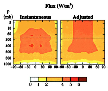
At least the IPCC informs us about three types of radiative forcing. This differentiation will be helpful in what is to come.
- Instantaneous forcing; ignores all changes in atmospheric temperature profiles
- Adjusted Forcing; allows for the (fast) adaption of the stratosphere
- Effective forcing; also allowing for the adaption of the troposphere. It should be very similar to forcing pv. Note: this will not include changes in the lapse rate due to WV
The Reconstruction
In order to get a proper handling on the subject, we can not rely on the IPCC, but instead we will have to explore some specific literature. One very useful paper here would be Myrrhe, Stordal 1997 - “Role of spatial and temporal variations in the computation of radiative forcing and GWP” (MS97)1. There Fig. 2 gives us the instantaneous forcing for a (minimal) CO2 increase from 356 to 361ppm. Usually such calculations are based on a doubling of CO2, but that is no problem. Given the logarithmic nature of CO2 forcing, we only need to consider this basic relation:
ln(2) / ln(361/356) = 49.7
As compared to the small CO2 increase they name, a 2xCO2 will provide a forcing 49.7 times stronger.
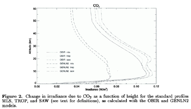
The first thing to check here is the question if these data can be reproduced. I took on the quite annoying work of going through the different data points manually in modtran. That means different altitudes, different CO2 concentrations in different scenarios and writing down both up- and downwelling radiation figures. Here is what I got..
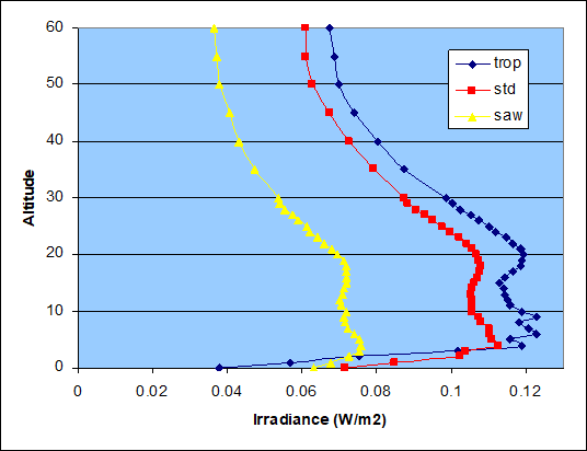
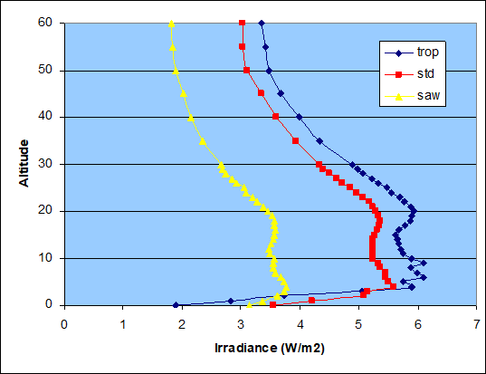
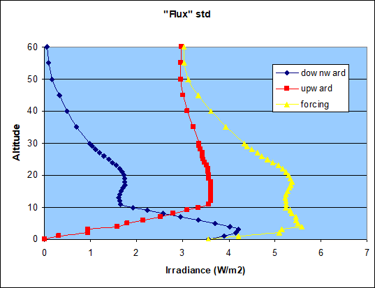
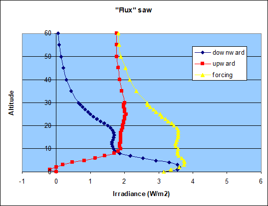
Although it is not a perfect match, which was not to be expected, it comes pretty close. Let me discuss a couple of issues. MS97 have three scenarios, tropical (trop), mid latitude summer (mls) and subarctic winter (saw). Since mls and trop are quite close by anyway, I dropped mls for a US std (std) scenario. Next modtran obviously suffers a little from poor resolution here, which is why lines tend to seesaw within the troposphere. Also the figures I took were for a doubling of CO2 from 400 to 800ppm, I only downscaled the results by the named factor of 49.7.
Sure it will be worth a look on the actual 2xCO2 forcing result. The forcing here would be about 5.3W/m2 at the tropopause level with the US std model. Obviously it will be more with the tropical scenario and less in higher latitudes, but on a global average that evens out. So the instantaneous forcing would amount to some 5.3W/m2.
Let me instantly address the confusion that may arise from this. I claimed that 2xCO2 forcing was a mere 2W/m2, consensus claims some 3.7W/m2, and now this indicates 5.3W/m2. How comes? This calculation is excluding clouds which will reduce the forcing to about 4.1 to 4.2W/m2. The other subject is the “instantaneous forcing”, meaning the stratosphere is yet too cool which will mean less “back radiation” from above and thus less forcing all over. Although I can not reproduce this stratospheric adaptation, a final result of some 3.7W/m2 might seem quite reasonable in this context.
So in a way we can reproduce the consensus estimate. Opposite to what I have stated before, the difference to my previous estimate is not due to “the science” ignoring overlaps, but because of the addition of up- and down “fluxes” at the tropopause level. Indeed we should have a closer look on those two components presented in the three charts (for each scenario) below.
Some Details
In this section I will explain why those curves look the way they do and what these data actually mean. I guess some readers might find this a bit too detailed and confusing, so feel free to skip it. Yet it is valuable information to understand the whole thing, so you might study it in detail, or draw your own conclusions from the data presented.
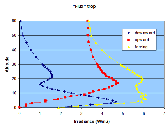
Downward Flux
Let me first discuss the distinct shape of the downward “flux” and we will start from the top. As you may imagine beyond a certain altitude there will be no LW “back radiation” as there is no, or too little atmosphere left. Naturally at 60km altitude a doubling of CO2 would have almost no effect in this regard. As we go down the stratosphere “back radiation” and accordingly enhanced “back radiation” gradually increases and preliminarily maxes out at about 20km altitude, a bit higher in the tropics, a but lower in high latitudes.
From there on the “flux” decreases. Why? As we approach the tropopause temperatures reach a minimum. Lower temperatures mean less radiation. The fact that there is more radiation from higher up does not help, as most of that will be (re-)absorbed before reaching these lower altitudes, or the tropopause respectively. Also one needs to consider here the tropopause is high in the tropics (~17km) and low in high latitude winter (~8km).
Below the tropopause “back radiation” increases both due to an ever denser atmosphere and higher temperatures. Accordingly the “downward flux” due to 2xCO2 grows rapidly. Yet, in the data above, this trend reverses sharply at below 4km altitude. The reason hereto is the increasing overlap with WV. WV is naturally highly concentrated in lowest layers of the atmosphere. Also it is a function of temperature. This kind of closes the atmospheric window and mitigates the role CO2 plays within. Accordingly in the inner tropics at surface level, a doubling of CO2 will have a minimal “back radiation” effect. With colder temperatures and less overlaps, the CO2 effect remains relatively strong.
Upward Flux
The “upward flux” by comparison is relatively simple, and this time let us go bottom up. At gound level CO2 will not change upwelling (surface) radiation. Bear in mind we are still talking “instantaneous forcing”, not allowing for any changes temperature. Only as we ascend within the troposphere, higher CO2 concentrations can take effect by gradually shifting the emission altitude upward into colder atmospheric layers, thereby reducing emissions.
Again the tropopause serves as a turning point, as from there on temperatures increase. Higher emission altitude combined with increasing temperatures means more emissions. As the “upward flux” is defined as less emissions, it shall be no surprise this “flux” decreases with altitude. Btw. if you wonder why the “upward flux” turns negative at 1km altitude in the saw scenario, it is due to inversion.
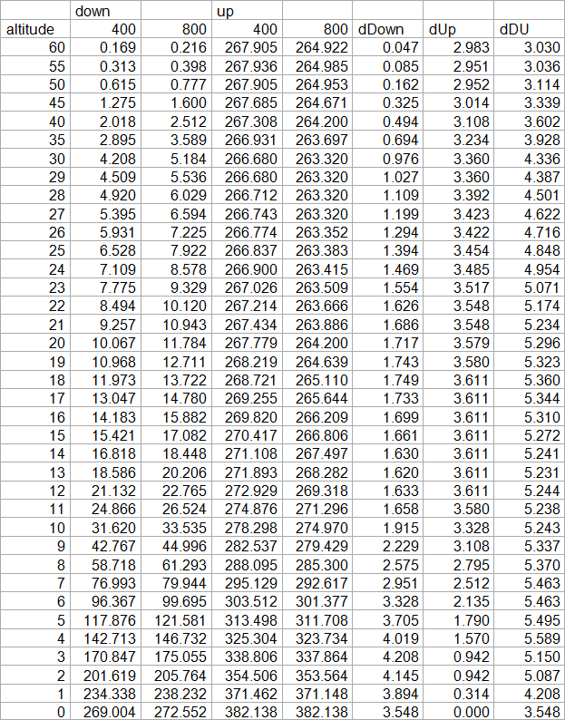
Next let me give you the “raw data” on up- and downwelling radiation (W/m2) with US std scenario (400/800 meaning ppm of CO2, dDown – downward “flux”, dUp – upward “flux”, dDU – delta up and down..):
All these data and details are meant to provide basic information on what is inside of the “black box”. This is indeed the “instantaneous forcing” as it has been used by the orthodoxy for decades. It is the very core of the “settled science” and it would seem few people know about it. And of course MS97 would not be the only source for this, Hansen et al 1997 (H97)2 would be another example, plus many more. I just do not have the time to read them all.
The beautiful thing about identifying and reproducing these results is that we can start a discussion and put them into perspective. You can not reflect on, criticize or falsify what you do not know. But now that we do know, we have a lot of means at hand. Remember, this is just the “instantaneous forcing”, but it serves as the basis to calculate “adjusted forcing” and “effective forcing” thereafter.
Discussion
1. General confusion
Looking at some of these papers, you start to wonder if the venerable climate experts know what are talking about. Here is an excerpt from Fig.2 in Hansen’s paper. It shows how, among others, the stratosphere is supposed to adjust. The problem is, the adjustment goes the wrong direction. With additional CO2 the stratosphere is supposed to cool, not heat. Although James Hansen is 82 now, he was 56 when the paper was published, so age will serve not as an excuse.
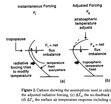
Also the inflated use the already ill fated term “flux” is not helping with building confidence. As explained you should not call radiation “flux”, because in most instances nothing will flow, not even heat. But then the named paper does not distinguish between the concept of radiative forcing and flux, as in the excerpt from “Plate 2” below. This is specifically absurd given the radiative forcing, as it is defined, adds up a decrease in upwelling and an increase in downwelling radiation.
And another example from Andrew Dessler3:
“lapse-rate feedback,” a negative feedback that occurs because a warmer atmosphere radiates more power to space, thereby reducing net surface warming.
Umm, no! What he is describing is the so called “Planck feedback”, not “lapse rate feedback”, and both are not really feedbacks btw. “Lapse rate feedback” is about the increase of latent heat transported by WV up the atmosphere, thereby reducing the lapse rate. “Planck feedback” on the other side has nothing to do with it.
I run into a lot of examples of this kind and these are not just typos, rather they point out a more profound problem. Leading climate scientists do not really seem to know what they talk about. I have the impression they just hold on to climate models, quote them, but otherwise have poor understanding of what actually goes on inside these models.
2. The logical discontinuum
I named it above, the enhanced GHE must obey to the same physical and logical rules as the basic GHE. As the name suggests, it is the same thing, only enhanced. For the sake of argument let us recall that Gavin Schmidt paper from 20104 (S10) and the attribution there. For instance for CO2 it states 21.7W/m2 SFR (or net, = 14% of 155W/m2) contribution and 38.1W/m2 SFR (or gross, = 24.6% of 155W/m2). We already discussed the importance of considering overlaps and why that will mean two different figures in terms of attribution of the GHE to its individual constituents.
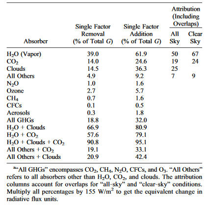
Evidently this follows a straight forward definition of the GHE, surface minus TOA emissions, like 394 – 239 = 155. And of course we can reproduce these figures with modtran. For a concentration of 400ppm in the US std model, we get 34.9W/m2 SFA (or gross) and about 20.5W/m2 SFA (or net). I discussed all this in far greater detail, also considering realistic surface emissivity figures, but that is a different story. The reason why modtran in this scenario produces lower figures, is that it assumes lesser surface emissions than S10 (381W/m2 vs 395W/m2). With less radiation to “shield”, not just is the GHE is smaller, but also the contribution by its constituents.
Percentage wise however it is an excellent match with 14.4% (=20.5/142) and 24.6% (34.9/142) respectively. That is despite my “quick and dirty” approach here. In fact, as you may imagine, the share of CO2 within the GHE is one of the largely settled questions and by and large I have no objections here. All great.
The problem we run into here, is that CO2 forcing must be CO2 forcing, regardless if we put something on top of it, or just look at what is already there. At 400ppm, again with the US std model, at the tropopause (12km) the SFA upwelling radiation SFA is 34.9 and downwelling radiation is another 12.4W/m2, or 47.3W/m2 combined, corresponding to a 33.3% of the GHE. SFR the respective figures are approx. 21W/m2 plus 12W/m2 with a total of 33W/m2, corresponding to 23.2% of the GHE.
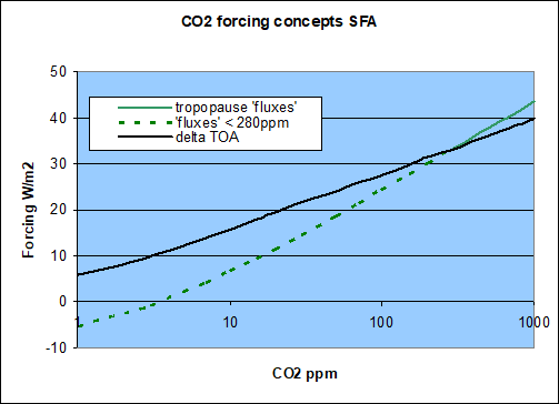
Let us take a closer look on that. I went through all these figures in modtran, both SFA and SFR. The black line here the “linear” logarithmic forcing you get TOA (top of the atmosphere). The logarithmic shape gets lost at very low concentrations btw. The green line on the other side is the sum of the both “fluxes” at the tropopause level. It is solid above 280ppm because that is where it turns into a GHE enhancing “forcing”, but dashed below, because there it would (re-)define the natural GHE, and this is not the way it is used within “the science”.
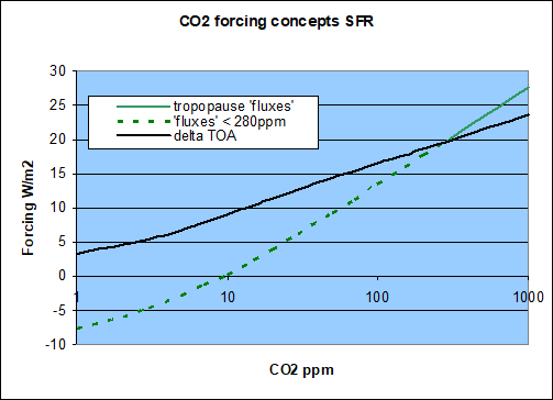
There is yet a little inconsistency here as modtran will not adjust the stratosphere temperature profile. So the green line represents the instantaneous, not the adjusted forcing. Let me quote H97 to point out the quantitative difference.
If the amount of CO2 in the air is doubled, the atmosphere becomes more opaque, temporarily reducing thermal emission to space. The instantaneous flux change at the tropopause is about 4.7 W/m2, but the flux change at the top of the atmosphere is only about 2.6 W/m2, because the added CO2 helps the stratosphere radiate to space more efficiently. The flux change at the tropopause is more relevant to the expected surface temperature change, as shown by comparison to the adjusted forcing, which is about 4.2 W/m2
Indeed the adjusted forcing should be about 12% lower than the instantaneous forcing in the SFR instance. In the above SFR chart the green line corresponds to 4.27W/m2 for a doubling of CO2, reducing it by 12% gets us to 3.76W/m2, the all familiar common consensus magnitude. But then why does H97 name 4.2W/m2? It is because an evolution occurring between SAR (1995) and TAR (2001), reducing CO2 “fluxes” all over. To quote TAR:5
IPCC (1990) and the SAR used a radiative forcing of 4.37 Wm−2 for a doubling of CO2 calculated with a simplified expression. Since then several studies, including some using GCMs, have calculated a lower radiative forcing due to CO2. The newer estimates of radiative forcing due to a doubling of CO2 are between 3.5 and 4.1 Wm−2 with the relevant species and various overlaps between greenhouse gases included
Anyway, the difference between the two lines here is not just 12%, but about 50%. While the TOA related forcing is only 2.15W/m2 (as before, without considering the surface emissivity discussion), the adjusted “flux” related approach gives us 3.76W/m2. It is a large and significant difference and only one of those two approaches can be correct. We are left with two options.
a) We can stick to the GHE as it is usually defined along with the attribution as named above by Gavin Schmidt. Yes, I have my objections to this as well, and for good reasons, but that is another story. Then however we need to reject the forcing concept current climate models are based on. Then CO2 forcing will drop to 2.15W/m2 only, and eventually 2W/m2 considering surface emissivity, and climate sensitivity will eventually settle at some insignificant 0.5K.
b) We can stick to the tropopause “flux” concept, but then given, or natural CO2 levels must necessarily play a much larger role in the climate of Earth. Also the attribution as presented above would be false and would need to be reworked. However, given the share of CO2 within the GHE is quite certain, this seems a bit unrealistic. Rather we would have to consider a larger GHE all over. And I am saying that in the context of the common GHE of 33K or ~150W/m2 being exaggerated already.
Now arguing a larger GHE is not a big deal within “the science”. In fact Manabe, who layed a lot of the foundations (and assumptions) of climate models, suggested a “radiative equilibrium” GHE of some 77K, as in the chart below (Fig. 4 – Manabe, Strickler 1964)6
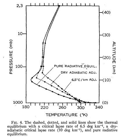
A model contradicting reality and telling us Earth should be 45K warmer than it actually is, might possibly raise some doubts. The issue was “fixed” by hard-coding a 6.5°C/km tropospheric lapse rate into the model. According to the authors this shall represent the escape of heat by convection. Safe to say this is not the utmost elegant approach. Moreover, once you add the restriction of outgoing radiation must equal incoming (solar) radiation, this “feature” alone will assure model output will not be too far off reality. In other words, the model will turn highly garbage-tolerant. Of course the multi-layer GHE is indeed nonsense and could be used as blue print to build a perpetuum mobile, if it worked.
Anyway, the point is, if the radiative GHE was even larger than the common 33K, then for some reason it would obviously fail to materialize, as the Earth is just as warm as it is. You may blame this on convective heat loss, or anything else. However you will not be able to explain, how this loss of heat would only affect the natural GHE, but exempt the enhanced GHE. Rather this enhanced GHE, or the radiative forcing causing it, will equally need to be discounted by at the least the same rate of heat loss. And that gets us back to where we started. Even enlarging the GHE will eventually have no merit in justifying the tropopause-“flux” based forcing concept.
It turns out whether opting for a) or b) will not matter. The discontinuity problem is severe and unless there should be a very creative “work around”, which I can not imagine, it is a valid falsification.
3. Another back radiation issue
As pointed out many times already, “back radiation” will almost always and almost entirely be cancelled out by “forth radiation”, meaning there will be no “flux” of energy or heat. When it comes to “back radiation” from the stratosphere however, there might be a logical window of opportunity, if you will. You could consider the stratosphere an autonomous, independent entity orbiting Earth in a way. If the stratosphere temperature wise is independent of what happens below, then it might potentially serve as a source of energy, just like the sun.
In reality however the stratosphere is not detached. The fact that temperatures change only gradually with altitude, rather than abruptly, reminds of us of it. Also there is something we easily oversee the way we apply radiative transfer models. If we split up the atmosphere into layers, for every kilometer of altitude for instance, and then increase CO2, very single layer will emit more radiation (and absorb more btw.). If for instance we set the tropical tropopause at 17km atltitude, then the layer 17-18km will emit more radiation downward, and the layer 16-17km will emit more radiation upward.
At the first glance this may seem contradicting, since we know the upward flux from the atmosphere will rather decrease. That is because the emission altitude increases, moving towards colder layers. But looking at it layer by layer, we get the opposite result. Given that most CO2 emitted radiation does not travel very far, but gets re-absorbed by other CO2 molecules nearby, what happens is that the layers just above and just below the tropopause (or even within the tropopause) simply just exchange more radiation.
This will also explain the “fate” of most of the “radiative downward flux” from the stratosphere. It originates just above the tropopause and ends just below it. Also it will be largely compensated the upward “flux” from below, so that we have a kind of “flux compensation” (sorry, could not help it). Anyway, it is hard to see how this would have any effect on the atmospheric temperature profile around the tropopause, let alone affect the whole of the troposphere.
4. How does WV feedback fit into this scheme?
To be honest, I still have no clue how “the science” argues a 1.8W/m2 WV feedback. You can find the figure, or a corresponding range of estimates (1.5 to 2.0W/m2) in many places, but I have not run into a conclusive rationale to it. I am still searching though. Once again the hints point to Mr. Manabe and his early modelling approach (MW67 is Manabe, Wetherald 1967)..
Values of equilibrium climate sensitivity near 4 K, the high end of the one-sigma range in the Sixth IPCC assessment (2.5–4 K for doubling of CO2; Forster et al. 2021) would be far less likely in the absence of a water vapor feedback comparable to that obtained by fixing relative humidity. MW67 is thus justly celebrated as laying the foundation for all estimates of the severity of global warming.7
Some interesting wording here. Let me add another quote from Dessler8..
A strong and positive water vapor feedback is also necessary for models to explain the magnitude of past natural climate variations
Let us understand the context here. First there is the knowledge over past climate changes - ice ages, warm or interglacial periods, you know. Second there is the idea of CO2 being a greenhouse gas, which it is btw. The idea is supported by ice core data showing strong correlations between CO2 levels and climate. Also you just have to look at Venus, with its massive and super CO2 rich atmosphere, causing a “run away GHE”. The scientific challenge now is to combine the two and explain past climate changes with variations in CO2.
This could be very straight forward, but it turned out not to be. The moderate variations of CO2 between roughly 200 and 280ppm through past ice age cycles will only produce a delta forcing of about 1W/m2 TOA. Temperature wise this corresponds to some 0.3K, which is about as much as the Earth cooled between 1940 and 1970, according to some earlier temperature records. That again led to some predictions of an immanent ice age, as you may recall, but I digress. It is fair to say linking CO2 to natural climate cycles was a far shot, long before it all become political, because radiative transfer models indicated CO2 was way too insignificant.
Taking a closer look even those “hints” were actually no good. From ice core data we know CO2 followed the temperature instead of leading it. The atmospheres of gas giants show similar temperature profiles as Venus, despite consisting mainly of hydrogen and being basically void of CO2. As GHG they only hold some minor amounts of Methane, something considered a “fossil fuel” by Earthlings. Yet at the respective pressure levels, they feature GHEs comparable to those of Venus.
If you think about it, it seems somewhat insane, as we are talking about 1 to 20 relation roughly. We do not really know by how much the climate oscillated, since we lack proxy data from the tropics and there is a chance climate barely changed there at all. But if we assume some 6K for global climate and compare it to the nominal 0.3K we get for CO2, it is just out of reach. Yet this was the objective and any move forward with the CO2 theory would require a massive amplification of its climate potential. The “flux” based approach discussed above serves one part of it, but a lot more would be needed. That is why a “strong and positive water vapor feedback” is necessary and a foundation for the “severity of global warming” (aka doomsday scenario) is “justly celebrated”, not questioned.
As far the questioning goes, I already discussed how vapor is unable to produce a primary feedback even close to 1.8W/m2 TOA. My estimate was, and still is, 0.65W/m2 after allowing for clouds and realistic surface emissivity. Effectively this will have less significance than the increase in latent heat, the consequential reduction in the lapse rate, and the reduction of the entire GHE due to it. “Climate science” calls this the “lapse rate feedback” and treats it like a real (negative) feedback, which it is not.
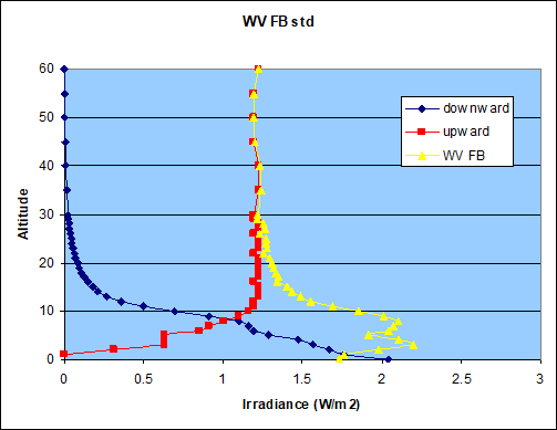
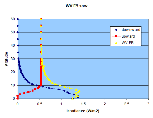
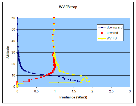
Now let us look what to get if we apply the “flux” approach. That is not even to say this was the way “the science” does it, because I still do not know. We only know the actual effect on emissions TOA by WV feedback is otherwise far too small and so we will need to consider this “logic”. Also since radiation is radiation, regardless if caused by CO2 or WV, the same physics should apply. The data below show the “instantaneous feedback” as analogy to the instantaneous forcing discussed above, excluding overlaps with clouds and surface emissivity corrections, for three different scenarios (tropical, US std and subarctic winter).
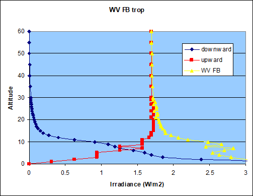
Due to insufficient resolution, as before, we again encounter the seesaw issue within the troposphere. Other than with CO2, the upwelling “flux” is barely changing from the tropopause upwards. This is because there is just not enough WV in the stratosphere to make a relevant difference. Thus the results from my analysis on WV feedback with regard to emissions TOA equally hold true for the upward “flux” at the tropopause.
Remarkably only the (inner-) tropical scenario is able to produce a 1.8W/m2 of combined “fluxes” at the tropopause (~17km altitude). All other scenarios will naturally fall short of this, with the US std yielding 1.5W/m2 (@12km) and subarctic just about 1W/m2 (@9km). A global average of 1.5W/m2 would be substantially less than the canonical 1.8W/m2, but still fall into the typical uncertainty range of 1.5-2.0W/m2.
Yet this approach has no merit in reproducing the consensus estimate. Once we allow for clouds that will reduce the upward “flux” by about 40%. As a principal showcase let me demonstrate what effect the simple “Altostratus Cloud Base .66 Top 2.7km” cloud scenario has on the tropical “fluxes”. Not just will those “fluxes” nullify within the clouds (below 2.7km altitude), as they already saturate the atmosphere with radiation, but the upward “flux” will drop from about 1.7 to only below 1W/m2 higher up, again a reduction of over 40%. In this regard it will not even matter what kind of cloud scenario we use, or how complex it is, rather it is predominantly a quantitative effect. Let remind you at this point, that clouds are responsible for about ½ of the total GHE in any way, considering their SFA or gross impact. Since their occurrence is correlated with that of WV, the overlaps are naturally massive. The CRE of the chosen cloud scenario is still well below the average CRE in the inner tropics btw.
Besides this, we would also need to consider the surface emissivity issue, the implicit overstating of the GHE of WV that comes with it, and of course these are just the instantaneous “fluxes”. As the stratosphere would cool, due to CO2 rather than WV, an increase of downwelling radiation from the stratosphere is not to be expected. All these factors combined, on a global average, the tropopause “flux” concept will hardly produce any stronger feedback, than the straight TOA approach already discussed. How “the science” comes to some 1.8W/m2 WV feedback, thereby making it a strong positive FB, potentially doubling the warming by CO2, remains a mystery.
As this point I can only speculate. Within the troposphere those “fluxes” are a lot stronger, so maybe that was the “inspiration”. Alternatively at surface level with clear skies, WV feedback will increase “back radiation” by about 4.3W/m2 in the inner tropical, and over 2W/m2 in the US std scenario. We know Manabe, and most of “the science” with him, erroneously believed “back radiation” was a source of energy, or heat respectively. If then the auto-generated heat by back- and forth “radiative fluxes” transcends via the hard coded lapse rate up the atmosphere, a lot of things can happen in model land. We are talking science fiction here, and not the good one.
5. The settling science narrative
“Climate science” loves to tell history in a certain way supporting its own legacy. Climate modelling has largely settled around some concepts introduced by Manabe and comrades. The narrative is that by then, the science had progressed so far that only details would need to be fine tuned thereafter. Already with preceding works there would have a convergence towards a certain consensus. Let me quote a certain A. Berger from Louvain8 on this, because it is a typical summary.
One century later, the development of the greenhouse theory took a new dimension. Plass (1956) calculated that the mean global surface temperature would increase by 3.6°C if atmospheric carbon dioxide doubled. Möller (1963) provided the first model attempt and suggested that water vapour might also act as an amplifying climate feedback mechanism. In 1967, Manabe and Wetherald provided quantitative results for carbon dioxide induced warming on the basis of a one-dimensional radiative-convective model.
It reads like a smooth evolution. But what did Plass and Möller actually say? Let me start with Plass9:
In order to obtain the temperature change it is also assumed that an additional amount of radiant energy equal to 0.0033 Cal cm-2 min-1 would be radiated to space, if the average temperature of the earth's surface were to increase 1°C...
When the CO2 amount is doubled and halved the change in the downward flux at the surface of the earth is 0.0119 and 0.0125 Cal cm-2 sec-1 respectively. Thus, in order to restore equilibrium the surface temperature must rise by 3.6°C if the CO2 concentration is doubled and the surface temperature must fall by 3.8°C if the CO2 concentration is halved.
I will have to explain that Calorie issue. 0.0033 Calorie per cm2 per min equals 1980 Calorie per m2 per hour (= 0.0033 x 10000 x 60). One Watt equals 860 Calorie per minute. And so 1980 / 860 = 2.3W/m2. The Calorie per second below is a typo, it meant to be per minute as well. Then it follows the CO2 forcing here is 0.0119 x 10000 x 60 / 860 = 8.3W/m2, and 8.3/2.3 = 0.0119 / 0.0033 = 3.6K.
Plass was not just totally off with his estimate in terms of forcing, also his logic over the “downward flux” (aka “back radiation”) is unrelated to actual CO2 forcing. So while the 3.6K figure looks like a totally consistent modern day estimate, as the IPCC tries push ECS a little northward of 3K, it is a totally unrelated, wrong and meaningless random number. Plass did not know how to calculate climate sensitivity. The only reason he gets quoted in retrospect, is that it superficially looks good and gives the impression of an ever growing consensus.
Also this example has a funny twist, if we are consequential with the “logic”. If you consider the additional “back radiation” as a source of heat, rather than the meaningless increase in back- and forth radiation between surface and atmosphere it actually is, you run into a runaway “Planck feedback” loop. The 3.6K temperature increase will not just effect the surface, but also the atmosphere above, increasing “back radiation” by over 5% (= ((288 + 3.6) / 288)^4). That would be about another 17W/m2 of “back radiation”, heating the planet by about 7K, causing even more “back radiation”, and so on. The cycle would go on indefinitely and turn Earth into a bright star. Once you introduce free energy, you can not contain it.
The weirdest and most telling aspect though, is that he got a “desirable” figure with the wrong means. This happens, when you first set the target and then try to figure out a way to get there. This is perfectly fine in engineering, but in any field where you are supposed to be guided by the evidence, without bias, it is a disgrace.
With Möller, who collaborated with Manabe, we have a similar situation, though for a different reason10:
It is shown, however, that the changed radiation conditions are not necessarily compensated for by a temperature change. The effect of an increase in CO2 from 300 to 330 ppm can be compensated for completely by a change in the water vapor content of 3 per cent or by a change in the cloudiness of 1 per cent of its value without the occurrence of temperature changes at all. Thus the theory that climatic variations are effected by variations in the CO2 content becomes very questionable.
It seems like he rather rejected the whole CO2 theory. Yes, he was a climate denier, though the term was not used back then. In both instances, and many more, it is highly selective cherry picking to shape something otherwise not existing. It is, in many ways, the equivalent to a witch hunt, where every accusation will get endorsed, no matter how unsubstantiated, but any exoneration ignored. Or in the age of TikTok videos think of a collection of skill shots where every single one hits. It is easy to do, if you cut out all the misses. It is all meant to create the illusion of confidence and certainty, when actually it was (and is) all vague.
Manabe was by no means perfecting the science, because it was still in its infancy. People did not understand the physics of climate, and neither did he. What he managed to do however, was to provide algorithms that would give seemingly reasonable results (most notably by hard coding the lapse rate), and a desirable climate sensitivity. That it seems, was enough to freeze and “settle” the science around this core.
6. The Hot Spot
This is something that struck me during the research hereto. The tropical hot spot is supposed to be the place of the strongest warming, next to the poles in theory, and the North Pole in practice. The explanation for it would be quite simple. As the atmosphere warms there will be more WV, along with more evaporation and more condensation. As discussed this means more heat transported from the surface up into the troposphere, thereby shrinking the lapse rate. Accordingly the (higher) troposphere must warm relative to the surface. To me this appeared fair and logical enough.
However, while doing this research, I realized what I named in point 1, that is people do not really seem to know why models behave like they do, and possible do not even care. Rather they just comment it, based on their own perception. Notably the instantaneous forcing based on the “flux” approach already produces a tropospheric hot spot, without even including any effects by WV. Then once the stratosphere is allowed to cool, the hot spot remains even more accentuated. There is a good chance the “hot spot” is rather an artefact of the “flux” concept, rather than primarily due to changes in the lapse rate.
Conclusion
Sorry for transpiring a lot of thoughts and concepts here. “Climate science” does things in a certain way and if we want to understand what is going, we need to follow it down the rabbit hole. To my knowledge, there has been no or barely any critical discussion over the “flux” concept so far, arguable because it is way too inaccessible and unknown to a wider public. The one scope of this article is obviously to change this and make this core of “the science” more accessible and promote a broader discussion.
Until then I took the freedom to start the discussion right away on my own, since there a lot of identifiable issues. The equation radiation = flux (of heat) is a nonsensical logic, opening the gates to an endless stream of free energy sources. The GHE is a real phenomenon restricted by real physics, not an “anything goes” situation. “Climate science” historically was prone to incorporate such free energy mechanisms and thanks to the “flux” terminology, still is.
Furthermore the “flux” concept is surprisingly not a direct projection of the GHE, but rather something different. This is weird in many ways. Both in terms of physics as well as epistemology, the GHG forcings have to be derived from the mechanisms of the GHE. If this condition is not met, then we are talking about an unsubstantiated theorem. Then, even by its own “logic”, the “flux” concept will not provide any significant WV feedback, unless one heavily relies on “back radiation”. This is something we know Mr Manabe erroneously did and was probably to foundation to the claim WV feedback would roughly double the warming potential of CO2. Despite his theoretical framework obviously being wrong, this relation has not changed with time. Otherwise radiative transfer models do absolutely not support this claim. Instead all the data indicate total WV feedback (incl. LRF) is indeed negative.
All these problems are to be seen in the context of scientists trying to explain paleoclimate variations with CO2, in other words the CO2 theory. While it failed anyhow, as you will still need an external forcing, the theory could only fly, if you manage to dramatically enhance the otherwise unimpressive CO2 forcing. Incidentally that is exactly what certain scientists, presumably followers of the CO2 theory, relentlessly did.
Opposed to it there is alternative framework, with the notorious mistakes of “the science” fixed. We know Lambda is set way too high, we know clouds are not cooling but slightly warming within the natural “climate system” and linked to it, the role of GHGs is vastly exaggerated. Also we know, once we not just look on the LW side, but have integrated over LW and SW effects of the atmosphere, it only just adds about 8K to the surface temperature as “atmosphere effect”. You may want to look up the respective chapters hereto.
All factors combined, the direct evidence, the circumstantial evidence and framework, it is safe to reject the “flux” concept.
5WG1 TAR - 6.3.1. Carbon Dioxide
Comments (3)
Menschmaschine
at 17.09.2023"The reasons that the CO2 variations have so often been assumed to be causes of climatic variations may be:
(1) The CO2 content of the atmosphere is so remarkably uniform over space and time that it is possible to observe long-range variations in its mean value. This is impossible for almost any other factor which can influence the radiation processes. Cloudiness, water vapor, and temperature show strong variations with day, season, latitude, and between oceans and continents. Observations are so scarce over about 60 per cent of the earth's surface that a secular variation in these factors cannot be recognized. CO2 content is the only factor whose secular variation we know.
(2) The influence of CO2 variations on the long-wave radiation seems to be evident because its physical mechanism is relatively clearly understood. It is, however, much more difficult to interpret its meteorological meaning and effects."
PALLA Manfred
at 02.10.2023Peter Dietze
at 19.08.2024https://www.fachinfo.eu/dietze2018.pdf Fusion 2/2018, HITRAN, ECS
MfG P. Dietze