

Vaporizing Vapor Feedback part 1
The inclined reader of this site may have recognized things go a bit different here. To those who think to know “climate science” it may look like alien technology. I do not give much on opinions, not even my own. Neither I like to ask questions I can not answer. Rather I enjoy some narcissist pleasure over exploring and providing answers, simply because I can. You know greyhounds need to run, geniuses need to solve. It is the most natural thing. For sure “climate science” requires some deep penetrating, laser sharp analysis as opposed to some dilettante theory building, or “polar bears are doing well” arguments.
Like that we have come a long way already. CO2 does not have a lot of warming potential, in fact “climate science” is overstating it by a factor of 2. Vapor circumstantially is not a GHG at all and will by no means serve as a positive feedback, and so the idea of any significant global warming due to CO2 has been rejected already. But that is not enough, as there is an overkill of evidence all due to be presented. Also within the dialectic approach, it is amazingly important not just to present one position so to say, but to represent all positions and understand their foundations, so that all contradictions can be traced back to their origins. In this way there will remain no contradiction at all, only different base assumptions, some justified, some not.
So when discussing “water vapor feedback” we will first have to analyze and understand what the “consensus science” is based on. First we need to distinguish between primary feedback, and the “feedback loop” so to say. It is not complicated. Let us say for some reason or forcing temperatures went up by 1K, which would make the atmosphere hold more of the “GHG” vapor, which again would warm the planet by say another 0.5K, meaning the primary feedback. Since now temperatures go up by another 0.5K, there will even more vapor, arguably producing another feedback of 0.25K, to which will be a 0.125K feedback, and so on.
Eventually going through all the iterations here, a 50% primary feedback will result in a doubling of the original forcing. If x was the primary feedback, the formula 1/(1-x) – 1 will give us the total feedback. Notably if the primary feedback was 1, this would result in a division by zero. Semantically it would mean a perfectly unstable situation, where 1K (or any) forcing would lead to an endlessly large feedback. Imagine a knife incidentally balancing on its tip, with any breeze or wiggle causing it to fall. The chances for this to occur and prevail are zero. Equally it can not be true for the climate system of Earth. Circumstantially any primary feedback, or rather all primary feedbacks combined, must be a figure between -1 and +1. The table below shall give some oversight on the relation between primary and total feedback.
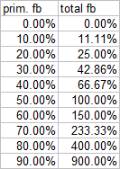
Obviously the difference between primary and total feedback is only moderate with low estimates, but turns hyperinflative with 50% upward. It is an important detail adding to the fragility of any feedback estimates. Error margins in the primary feedback estimate will necessarily multiply in the end.
So let us investigate what such primary feedback estimates are based on. Again I will use modtran1 to play through the different assumptions. First of all, since “climate science” likes to use a Lambda of 0.3 and usually ignores overlaps and real surface emissivity, I will simply follow along. With a temperature increment of 1K there should be roughly 6.5% more vapor in the air, so we just need to look up the impact on emissions TOA. That would be without any other GHGs or clouds respectively.

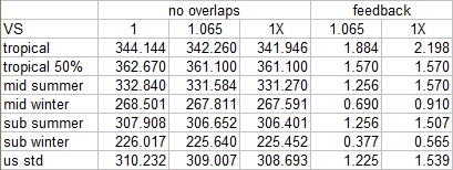
Most of the feedback would come with already high humidity levels, to be found with warm climate. In the inner tropics, with over 50mm of precipitable vapor, there would be 1.884W/m2 in primary feedback or 0.565K, and 1.3K total feedback. All other localities would stay well below a 100% total feedback, with very low figures for winter scenarios.
Without going through all possible weighting issues and considerations, it is well imaginable one could assume roughly a doubling of the original forcing by water vapor feedback. Sure there is only little feedback in the cold regions, while the tropics obviously have a lot of potential here. Then again one would yield even higher results with a surface emissivity of 1, other than the 0.975 or so modtran uses.
On top of that, if you include other (positive) feedbacks, like an alleged positive cloud feedback(!?), there will be cross-feedbacks providing the freedom to really model whatever you would like, without much scientific foundation. To keep things simple and rationale I will stick to vapor feedback to the original (CO2-) forcing. In this way we find relative good accordance with the status quo of “climate science”.
Thus, although there continues to be some uncertainty about its exact magnitude, the water vapor feedback is virtually certain to be strongly positive, with most evidence supporting a magnitude of 1.5 to 2.0 W/m2/K, sufficient to roughly double the warming that would otherwise occur.2
This statement refers to the primary feedback btw, as 1.5 – 2.0W/m2 would mean 0.45 – 0.6K with a Lambda of 0.3, and 82% - 150% of total feedback. And yes, we can understand what “climate science” is talking about, where the estimates come from, which assumptions they are build on, and why there is some implicit uncertainty. Building on the same foundations I would come to no substantially different conclusion.
The problem is, we know about a lot of flaws in those underlying assumptions and of course we are not going ignore them. First of all Lambda is NOT 0.3, and it will depend on emissions TOA anyhow. Not just Lambda would be different with different climates, but also if you ignore other GHGs and clouds you get higher emissions TOA, which effectively will lower “Lambda”. Let us see what happens if we ask modtran outright what temperature offset3 will be required to compensate the respective primary radiative feedbacks.
Note: VS 1 stands for vapor scale = 1, meaning the default modtran figure. Obviously with “tropical VS 0.5” it is just 50% of it, for reasons discussed here
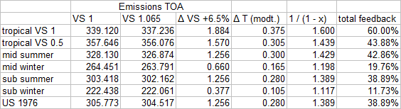
Modtran here basically follows the physics. For instance we can calculate ΔT with the US scenario ourselves. 305W/m2 means a black body emission temperature of roughly 271K. It then follows ΔT = (304.517/305.773)^0.25 x 271 – 271 = 0.28. Modtran has nothing up its sleeves here and only plays it fair. The difference to the erroneous approach above could not be more severe, as total feedback almost halved over the different localities.
The other main reason for this massive reduction, next to the Lambda issue itself, is in emissions TOA far exceeding real conditions. It is due to the absence of emission mitigating GHGs, cloud and real surface emissivity. A fact that points out the absurdity of “consensus” estimates, as they are ignoring these factors in terms of overlaps, and then apply the so derived forcings on real emission figures including them. Once we add other GHGs to the model and thereby include at least some overlaps, emissions TOA sink towards more realistic values, thereby mitigating the “Lambda issue”, but overlaps do dominate.
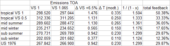
As the data show, vapor feedback is highly sensitive even to these small overlaps. Despite only about 10% of the vapor GHE is overlapped with other GHGs (excluding clouds!), allowing for it reduces total feedback by another 20% on average. Vapor feedback becomes ever less impressive when moving from a theoretical construct towards more realistic parameters.
The next iteration towards reality would be including clouds, which provide the largest overlap with vapor. It is a little bit tricky to pick the proper cloud scenario, as the different climates have different CREs (net longwave cloud radiative effects to be precise), while the available options within the uchicago modtran are extremely simplified and limited. Given the global (net) CRE should be 30W/m2, the chosen parameters are quite conservative. With the inner tropics for instance the CRE is well above the average, about 40W/m2.
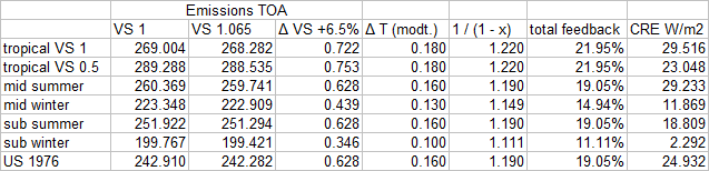
There is roughly only a 20% feedback remaining, and we are safely in the low regions where the feedback loop only plays a small role. Obviously the vapor feedback theory totally depends on wrong assumptions and instantly falls apart if real conditions are allowed for. Nothing else was to be expected. Just for illustration let me show how this looks like in modtran, based on the US std locality.
Yet, this is not the end of the story. As we have discussed there are complex issues to be considered with the simplistic cloud model modtran applies. Quantitatively these CREs are too small and thus will underrepresent overlaps, and thereby overstate the feedback. Quality wise the opposite is true, as one simple, low, opaque cloud layer will produce larger overlaps at any given CRE with vapor, than realistically complex cloud models.
Then there remains the gorilla in the room, meaning surface emissivity, which if accounted for not just halves the GHE of vapor, but equally affects the radiative effect of any increment. With the Spectral Sciences4 “modtran web app” we can parameterize surface emissivity, though it is a bit flawed as I had to find out. The problem is, they have only one atmosphere temperature profile fitting the “mid-latitude summer” scenario, with a close to surface air temperature of 294.2K. If you switch to any other “atmosphere model”, the surface temperature changes and many other parameters as well, but the air temperature remains the same. For instance “sub-arctic winter” would have a ground temperature of 257.2K, but the air right above it would be 294.2K. The bug has been reported and confirmed, hopefully they are going to fix it soon. Till then it is mandatory to only use the “mid-latitude summer” scenario.
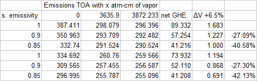
As with the uchicago version the default water column for this scenario is 36.something mm of precipitable vapor, or 3635.9 “atm-cm” as it is defined here. The output is restricted to WN 250 to 2.000 (5-40µm), representing 91% of the emission spectrum. Certain GHGs, N2O for instance, can not be parameterized. I ran the model with 0, standard and standard + 6.5% vapor columns vs. different surface emissivities. Although surface emissivity is about 0.91 globally, within the far IR, where the main vapor absorption is located, it is only about 0.875. Also as there is wavenumber limit of 250, a decent part of this main absorption band is missing all over.
As shown before, real life surface emissivity figures massively shrink the attributable GHE of vapor. The feedback to a 1K warming simulated by a 6.5% increase in vapor drops by 27% for 0.9 vs. 1 surface emissivity both with, and without other GHGs. A 0.85 surface emissivity enhances this to 40.6% without, and 42.1% with other GHGs. Considering the lacking part of the spectrum, the variation surface emissivity underneath the respective absorption band and weighting it accordingly, I can infer some 30-35% reduction in vapor feedback due to allowing for realistic surface emissivity.
This percentage will not simply be additive to the overlap effects discussed above. It is however fully applicable to the clear sky fraction and given the low and conservative CREs applied, primary radiative vapor feedback is most likely about 0.5W/m2 only (as opposed to some 1.5-2W/m2), corresponding to 0.135K primary, and 0.15K (or 15%) total feedback.
Interim Conclusion
The radiative vapor feedback potential in the sense of roughly doubling any forcing is a theoretical train wreck. Almost to its entirety it is build on simplifications and assumptions undue. Like with CO2 forcing, introducing realistic parameters has pivotal consequences. But unlike CO2, whose forcing potential gets halved, vapor due to the relatively low emission level it provides, is far more exposed to the named errors. The mandatory introducing of overlaps and surface emissivity thus causes a carnage and about 85% of the assumed radiative vapor feedback was never real.
Update 11.11.2021
Alright there is one thing I feel obliged to add, and furthermore change my estimate. I simulated vapor feedback with a 6.5% increase in water column increase. With ambient temperatures, a 6.5% increase per centigrade is perfectly plausible. As pointed out, vapor feedback is most significant in the tropics and there, with temperatures in the 25-30°C range, you should expect only a 6% increase. In fact WH20215 use a 6% increase in WV only to simulate WV feedback.
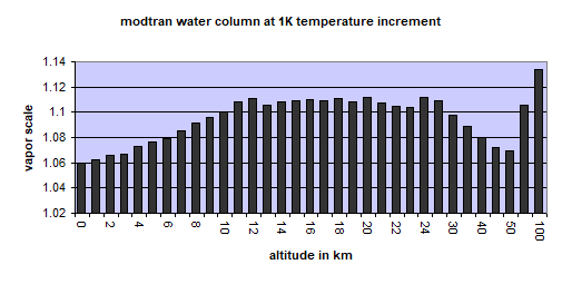
The issue I ran into is that modtran would in some odd way produce more WV feedback than I expected. Quantitatively there was no real disagreement, so the answer had to be elsewhere. What I found was a difference in the distribution of WV with regard to altitude. At high altitudes WV would increase by up to 11% due to 1K increase in temperature. Checking back with the Clausius–Clapeyron relation I found this might actually make sense. The slope of WV saturation is steeper with low temperatures, as there are at higher altitudes.
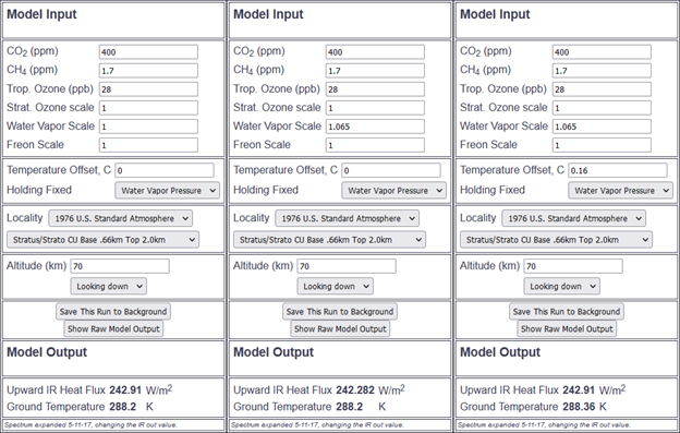
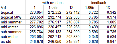
In order to investigate this reasonable(!) behaviour by modtran, I added a temperature offset of 1K in the first place. That is important, as only with a temperature offset holding relative humidity fixed will have any effect. Then there are three scenarios to be played through. The first one is just about adding a temperature offset of 1K while holding WV pressure constant. With the second scenario WV scale is increased by 6.5% to 1.065. In the third scenario, marked as “1X”, WV scale is back to 1, but this time relative humidity is fixed to allow modtran to increase WV according to its own parameters. The difference in emissions TOA with the two latter scenarios will give us the feedback in W/m2.
My previous assumption was this should make any notable difference, but obviously I was wrong. Despite some precision issues, well visible with the low humidity tropical scenario due to low resolution, modtran produces about 25% more WV feedback. It is not because modtran would add more vapor over all (6.44% vs. 6.5%), but due to a significantly stronger increment at altitude. Notably these results are in better accordance with the orthodox claim of a 1.8W/m2 primary WV feedback.
However, as discussed, such estimates are obsolete as they exclude overlaps. Adding other GHGs and some CRE (“Stratus/Strato CU Base .66km Top 2.0km” throughout, except for inner tropics where it is “Altostratus Cloud Base 2.4km Top 3.0km”), WV now trends towards 0.85-0.9W/m2 in the global average.
Yet, as before, these figures are based on low CREs and exclude the effects of realistic surface emissivity. Accounting for all of it I will raise my WV feedback estimate to 0.65W/m2.
3modtran is a bit "sticky" when setting a temperature offset and can produce identical emissions for a specific range. If so, the average figure is given
Comments (0)
No comments found!