As an undisputed basic fact of climate science, vapor is the most significant GHG, providing a strong feedback to any (exogenous) forcing. Regrettably this “fact” is utter nonsense and it only has been undisputed because no one had the brain to get it right. Let us change this for good.

I have dealt with this issue before, yet in order to discuss vapor feedback, we should have a deeper look on it. And I must admit in the course of doing so, it provided me with some interesting insights I did not expect. Let us first recall what Gavin Schmidt says about the GHE of vapor, since it pretty much represents the status quo of “climate science”. I mean he is as much establishment as it could be.

In the “Attribution of the present‐day total greenhouse effect”¹ we find vapor would account for 39% as “single factor removal” and 61.9% as “single factor addition” of the total GHE of 155W/m2. For simplicity the terminology can be changed into net, and gross GHE, meaning whether of you include overlaps with other GHGs and clouds, or not. And despite all justified criticism, or falsifications rather, which are up to come, it is quite remarkable to find overlaps with clouds even considered. Anyway this would result in a 60.4W/m2 net-GHE and 96W/m2 gross-GHE by vapor.

Given such numbers it is no surprise vapor is considered an almost almighty GHG, responsible for the bulk of the GHE. Interestingly this has lead a lot of “criticals” to argue CO2 was irrelevant, because vapor, you know. You might find totally absurd constructs² defying all logical and physical restrictions, which simply try to shovel GHE from CO2 to vapor, so that CO2 would turn irrelevant. The idea seems appealing. With vapor being the main culprit anyhow, if we put all the blame on it, CO2 might get an absolution. You might want to try this in a courtroom, but it will not work in physics.

Rather CSI “global warming” will have to take an unbiased look at the physics. Nothing seems more obvious than asking modtran. First let us examine the gross-GHE of vapor, by nullifying all other GHGs and comparing emissions TOA with, and without vapor. The uchicago version gives a “water vapor scale” (VS) of 1 for every respective locality, which is highly ambiguous. Accordingly I looked up the data behind the model to find how much vapor it actually assumes.

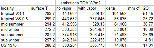
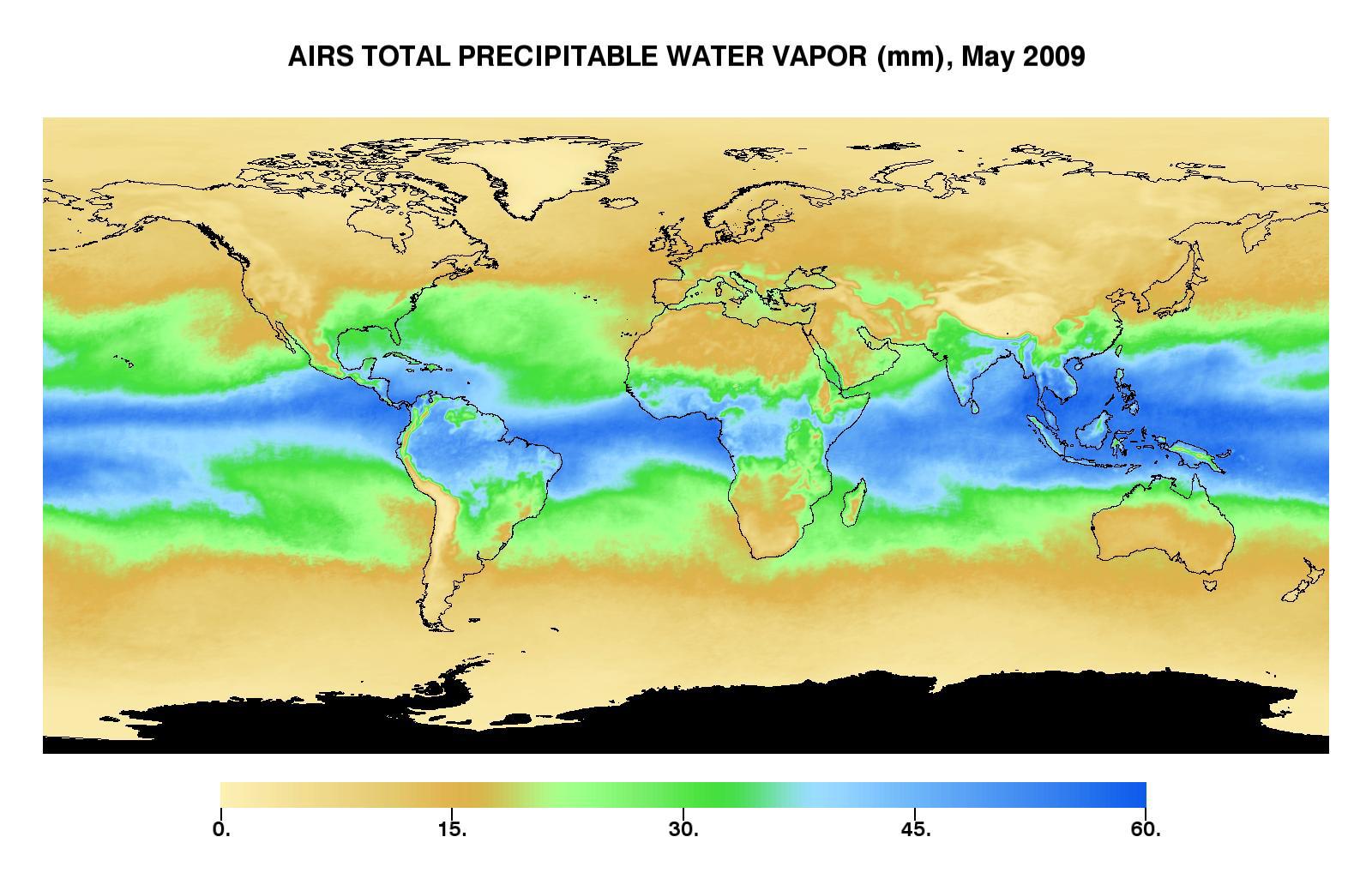
Other than CO2, with its uniform concentration all over the atmosphere, vapor is unevenly distributed. Accordingly modtran uses a wide range of different humidity levels over the respective localities. Given the complex reality, see the graph³ below, these are really just ballpark figures. And even though you can parameterize the “water vapor scale”, the question is up to which level? To properly assess the GHE by vapor you would a) need a lot of data on the actual concentration and distribution, and b) a complex computer model to process the data. Both is beyond my means.

However we can put the parameters used into perspective and make some simple comparisons. For instance the “tropical” locality with over 50mm of precipitable vapor represents the wet inner tropics, not the geographic tropics defined by latitude (between 23°26’S and N respectively), where it is mostly much drier with easily only half as much vapor, or less. Thus the 104W/m2 of GHE is the upper limit, an extreme not representing the geographic tropics, let alone the planetary average. Notably Schmidt’s estimate of 96W/m2 global gross-GHE comes very close to this upper extreme, suggesting it must be a considerable exaggeration.

Then there is another interesting detail in the results above. According to the model there is roughly a linear relation between temperature and vapor gross-GHE, with about 1.8W/m2 per K. Using the US std atmosphere as a pivotal point, this would give for instance 18.7W/m2 (=(257.2-288.2)x1.8+74.5) for “subarctic winter” and 95.2W/m2 for the tropics, close enough to the actual model output. Do not be afraid, I am will not try to derive a climate model from it. The point is rather, that given such linearity, a model using the global average temperature should be a valid approximation, which is a welcome and almost necessary simplification. I know it is not perfect, but using US std atmosphere as proxy will only introduce a small margin of error, as opposed to the large error margins we are going to discuss.

First of all, if we assume the US std model to approximate the global average with some 74.5W/m2 of gross-GHE, then Schmidt’s estimate will be over 20W/m2 too high. The biggest part of this difference can be explained by the inferred surface emissions. While it is only about 380W/m2 with modtran, Schmidt probably assumes some >390W/m2, a figure usually published by his employer NASA⁴, and necessary to conclude a GHE of 155W/m2. On the other side, if modtran was using perfect emissivity, it would also yield a higher gross-GHE, likely in the 83W/m2 region (actually 82.6W/m2 after looking it up).

The actual gross-GHE of vapor

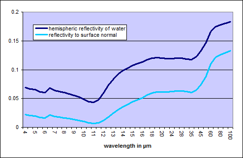
I will admit such considerations are extremely boring, so let us do something highly innovative and exciting. Since we have reasonable data on surface emissivity, as presented in the graph above, why not take them into account? Sure it is a bit complicated, but yet feasible. The merit is, we no longer need to compare model data on emissions against a perfect black body, but can do so against the real surface. Since we know satellites look straight down, and the model data are essentially a synthesis of these satellite- and some spectroscopic lab data, surface emissivity to normal should fit like a glove.

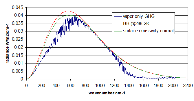
Something interesting is happening in the 600-900WN range. The erratic emission curve there is touching the green surface emissivity line many times, but never crossing it. It suggests that vapor is still highly transparent there and most of the effective deviation from perfect emissivity is not due to vapor, but rather due to the surface itself. Given this part of the spectrum houses the main CO2 absorption band (WN580-760), it would solve an old conflict. That is if there is a significant overlap between CO2 and vapor, which the models suggest, but spectroscopy to my knowledge largely denies. It all could be just an artefact within the model data, due to ignoring surface emissivity. A detail even I might have to (re-)consider.

Next and obviously, the difference between the blue and the green curve, which defines the GHE of vapor, is substantially smaller than that between the blue and the red curve. While the gross-GHE of vapor would be 82.6W/m2 with the red curve as benchmark, the figure shrinks to 67W/m2 with the green line, representing real surface emissivity (to normal) of course. The deviation here mainly affects the far-IR range, or low WNs here, while it has only little effect with high WNs.

The next problem is, despite surface emissivity to normal is naturally a good match for satellite data, we will actually have to consider hemispheric emissivity, which is a lot lower. In fact within the far-IR range it is only about 0.875 with water, and again, we have insufficient information on other surface types. If we plot hemispheric surface emissivity vs. modelled emissions with vapor, something may seem counter intuitive, as the blue curve will exceed that green curve. To understand why that is, and has to be, we always need to bear in mind the perspective bias by only looking straight down. It is not like vapor would add emissions here, rather it just dampens surface emissions with an optical thickness below 1, and in some lines even 0. Really it is just the hemispheric vs. surface normal issue, or what satellite can see vs. what it fails to see respectively.

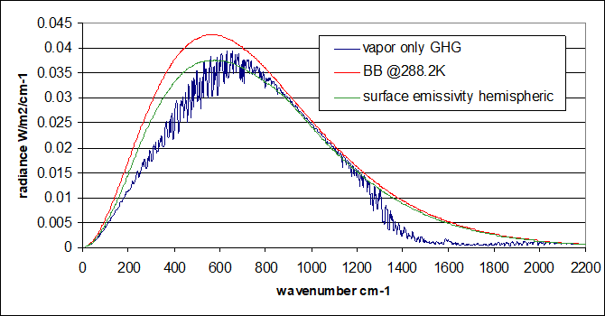
The important part here is the difference between the area underneath the two lines is only 46.5W/m2. Note the modtran output yet includes some minor GHGs which can not be parameterized, or set to zero. But they only account for some 1.7W/m2, which will be largely overlapped with vapor anyhow.

Compared to the 96W/m2 Gavin Schmidt names as the gross-GHE of vapor, 46.5W/m2 are not even half as much. It is a huge difference necessarily changing our understanding of the role vapor plays. Other than CO2, which attains very high emission levels within its main absorption band, vapor has wide absorption bands, but only provides a moderate elevation of the emission layer. Therefore ill fated assumptions on surface emissivity have a much larger impact on the attributable GHE, or the correction of those assumptions respectively.

The net GHE

Yet we are left with the question of the net-GHE of vapor, and it is a tricky one. The easy part is with other GHGs, accounting for some 10% overlap, a figure consistent with both the literature and modtran. It is just a relatively small overlap after all. With clouds it is a lot harder. The figures given by Schmidt are far off, vastly overstating vapor and understating clouds, so that there would be little merit in trying to extrapolate them.

With modtran at least we can get some more reasonable figures. With US std atmosphere and standard concentrations for other GHGs, vapor would add 67.2W/m2 (=335.038 – 267.842) GHE, roughly 10% less than without other GHGs. With a CRE of 25W/m2 this figure drops to 40.3W/m2 (= 283.197 - 242.91), and with CRE of 39W/m2 to 29.5W/m2  (=228,875 - 258,359). We can infer a CRE of 30W/m2 would give us about 37W/m2 of net-GHE for vapor within the model, about half of the 74.5W/m2 the model gives us without overlaps. Applying this ratio on the 46.5W/m2 gross GHE I calculated above, with the inclusion of real surface emissivity, we would infer some 23W/m2 net GHE.

Yet there are some significant issues to be considered, and these are the reasons why there remains a significant level of uncertainty. First of all, a CRE provided by one opaque cloud layer at relatively low altitude, as modtran does, is an insult to the complexity of real life cloud conditions. As vapor diminishes quickly with altitude, this will cause a bias overstating the overlap.

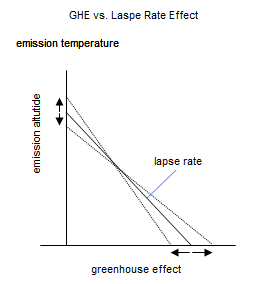
Secondly the model, build on high emissivity assumptions, will likely overstate the emission altitude of vapor. For instance, if a satellite measures emissions fitting a black body at 260K, this would be 28K less than a surface temperature at 288K, and with a lapse rate of 6.5K/km you would assume an emissions altitude of 4.3km. If the emissivity (of vapor and surface) was only 0.9, then it will take 267K for the same emissions, suggesting an emission altitude of 3.2km. On top of that, ignoring real surface emissivity, a lack of emissions will tend to be translated into colder emission temperature and an elevated emission level, as shown above. It is an innate problem of modtran, and likely hitran as well.  

Thirdly there is a bias by plotting average humidity against average cloudiness. In reality both are correlated and with dry come few, with wet air lots of clouds. For instance in the Sahara the air is very dry, meaning a relatively weak vapor-GHE given tropical heat, but for a lack of clouds an equally small overlap. In the inner tropics, with its abundance of high rising clouds, the overlap will be huge. It is well possible, even likely, that the net-GHE of vapor will be larger with dry tropical conditions.

The latter two points will necessarily cause an underestimate of the cloud-vapor overlap. Without proper assessments of these individual biases, weighing them against each other is a bit pointless. The 23W/m2 figure for the net-GHE established above might serve as an orientation anyhow. If higher in reality, it can only be by a moderate margin. More likely the net-GHE of vapor will be smaller, as already suggested. Either way, it is miles off the 60.5W/m2 net-GHE or “single factor removal” Schmidt named, thereby representing more or less the status quo of “climate science”.

Latent heat

Eventually we need to consider that vapor, other than CO2, is a condensating GHG, meaning another important property, as it is transporting latent heat. A “wet” lapse rate of 6.5K/km with the given mix of GHGs and clouds provide some 115W/m2 of total GHE. If we had a dry adiabatic lapse rate of 9.8K/km, with given GHGs, this GHE should be about 115 x (9.8 / 6.5) = 173W/m2, or almost 60W/m2 larger. Then this is a bit simplified since we would a) need to consider the GHE provided beyond the troposphere where the lapse rate is very different, and b) a dry lapse that should even exceed 9.8K/km, given a naturally unstable atmosphere. The indication is a dry, unstable lapse rate of about 10.8K/km2, meaning a latent heat effect of 76W/m2. Kiehl/Trenberth for instance name even 80W/m2 as latent heat effect⁵.

Although this figure easily exceeds that of the gross-GHE of vapor, we need consider the GHE of vapor itself is affected by it. So if vapor provides some 46.5W/m2 of gross-GHE with the given lapse rate, counterfactually it would be 70W/m2 (=46.5/6.5 x 9.8) assuming a lapse rate of 9.8K/km, and 77W/m2 with a lapse rate of 10.8K/km. That would be 77W/m2 of gross-GHE vs. 76W/m2 of latent heat effect. I am not saying they are exactly the same, but playing through the different assumptions it is obvious both would roughly even out, making vapor essentially climate neutral. That is in terms of surface temperatures.

In reality however it is not quite such a nail biter, as the variable components are the net-GHE vs. the latent heat effect. And of course with latent heat there are no overlaps, as vapor is the only responsible agent here. Also with latent heat, other than radiative forcings, we do not have “saturation”. Rather it does scale pretty well with the abundance of vapor. Adding it all up, there are mighty implications.

First of all, as latent heat dominates its radiative effect, vapor is not really a GHG. It works like heat pipe transporting heat from the surface to the emitting layers of the atmosphere. Effectively vapor is a net cooling agent, and anti-GHG, or if you will an air conditioner, for the simple minded. Sure an insight very disruptive in the context of “settled science”.

Secondly it is not amplifier of any exogenous forcing, but rather a mitigator. The modulating latent heat will necessarily outrun any modest ratiative forcing, or rather feedback if we stick to the given terminology, by a large margin. Vapor stabilizes the climate temperature wise, while being likely a very sensitive factor with regard to precipitation. Though that is another story. I am going to deal with the quantification of the respective effects in a later article.

This should help us understand reality. Why are deserts like the Sahara so hot on average? Obviously it should not be due to a) the lack of the “GHG” vapor, or b) the high surface albedo. Also it can not be due to c) few clouds, as they are definitely warming. Provided the correct understanding of vapor, it is due lack of it, or its net cooling effect respectively. Also it makes clear why we see no “footprint” of vapor with night time cooling rates, to name just two instances.

Summary:

The perceptions on the role of vapor within the GHE represent a dramatic failure in properly accounting for surface emissivity. Although this neglect does affect all GHGs, vapor with its relatively shallow emission level and wide band absorption range, especially prominent within the far-IR, where surface emissivity is specifically low, is most severely affected. The gross-GHE of vapor is easily exaggerated by a factor of 2, its net-GHE possibly even by a factor 3.

Although there remains some uncertainty, the net-GHE of vapor is within a similar magnitude as that of CO2. This insight is not only in stark contrast to “consensus” positions, but even more so to “critical” positions claiming some irrelevance of CO2, as vapor would dominate it as GHG by far.

Rather in the bigger picture, vapor is way more effective in transporting heat from the surface to the emitting layers of the atmosphere, than elevating the emission level and thus providing some GHE, so that it is cooling the planet. The fact that “climate science” gets this wrong, believes vapor would be a massive GHG instead of the cooling agent it actually is, documents well the dreadful state this pseudo-science is in.

¹https://pubs.giss.nasa.gov/docs/2010/2010_Schmidt_sc05400j.pdf

²Here I wanted to refer to a recent paper, which regrettably seems to have been revoked. I do not suppose my email pointing out its blunders had any influence on the decision.

³https://airs.jpl.nasa.gov/resources/174/global-total-precipitable-water-vapor-for-may-2009/

⁴https://www.nasa.gov/feature/langley/what-is-earth-s-energy-budget-five-questions-with-a-guy-who-knows

⁵https://scied.ucar.edu/learning-zone/how-climate-works/energy-budget