

Vapor Feedback II: The Lapse Rate and the Feedback Catastrophe
The “lapse rate feedback” is the other component of vapor feedback, and it is negative by nature. In order get a comprehensive understanding of vapor feedback as whole and ECS estimates, we need to explore it. The orthodoxy seems not just to lack an understanding of its magnitude, but also of its nature.
As discussed in the first part of this article the radiative effect of a 6.5% increment of vapor will only result in 0.65W/m2 forcing, rather than common estimates of 1.5-2W/m2. Forcing? Yes, if we would assume an endogenous increase in vapor that would be a forcing, if we assume an exogenous cause that will make it a feedback. Stupid terminology! It does not really matter, since it is all about the figures. Again, the difference between the orthodoxy and accurate estimates is all about the denial of overlaps and surface emissivity.
In reality the lapse rate is amazingly complex. It differs from place to place, differs with altitude (within the troposphere!), changes with day time and season, and also depends on the weather, or is even causing it respectively. The claim of one single lapse rate of 6.5K/km is an extreme simplification, just as an average temperature of about 288K is. Yet this simplification has its merits. As the average surface temperature, the lapse rate is not a random product. Despite the chaotic complexity of “weather”, it still follows basic physical rules. And if these rules, or rather the parameters change, the average lapse rate will change as well.
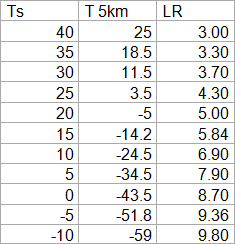
An emagram1 like the one below can easily cause eye cancer, so use it at own discretion. For those willing to take the risk it contains plenty of information. A perfectly dry and unstable atmosphere, which gets predominately heated at the surface, is assumed to have a lapse rate of 10.8K/km. A perfectly wet lapse rate however will get ever smaller the higher the temperature, which is due to ever more latent heat.
It is certainly not the most scientific approach, but reading out the data from the graph we can compare temperatures at the surface, and at 5km, roughly the average emission altitude. Due to the ever shrinking lapse rate, temperature @5km increases almost twice as fast as surface temperatures around the global average of 15°C. The relation however is smaller with lower and higher temperatures.
Initially I thought I could use this as a basis for further considerations, but then I realized that would be a mistake. As the emagram points out, pressure levels increase in altitude with growing temperatures. Of course, one might add, as a warmer air will expand, like with a hot air balloon. As the air expands, GHGs and clouds will equally increase their emission altitudes, which in opposition to the lapse rate effect, will increase the GHE. To allow for it, we should focus on pressure levels, rather than altitude. The average emission level of the atmosphere should be somewhere between 60 and 50kpa.
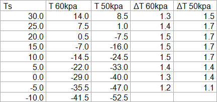
So the emission temperature should increase by about 1.6times the surface temperature, if the atmosphere was totally “wet”. Which it is not however, although an environmental lapse rate of 6.5K/km comes fairly close to a perfectly wet lapse rate (~5.8 @15°C Ts, ~5 @20°C). Relative to a dry, unstable lapse rate of 10.8, it leans about 80% to the wet in the global average. Applying this percentage on the 1.6 relation, the emission temperature should grow about 1.48times the surface temperature, corresponding to a 1 / 1.48 – 1 = -32.4% negative lapse rate feedback. Sure a casual approach, but it gives us some orientation.
I wanted to compare this figure to those given in the assessment reports of the IPCC, starting with the first. Regrettably searching the FAR for the term lapse rate did not yield any relevant result, which may be due to the poor quality of the scan circulating on the internet. And sure I do not want to read the whole damn thing. However the IPCC has referenced Hansen at al (1986)2.
If Fig. 6 scenario b Hansen suggests about 1.2K 2xCO2 forcing, 1.7 + 0.9K vapor feedback, 0.35K surface albedo-, and 0.85K cloud feedback. Vapor feedback here consists of two components, vapor amount and “vertical distribution”. A similar distinction is made with clouds, as cloud altitude- and cloud amount feedbacks. This would add up to an ECS of about 5K, only mitigated by some -1.2K lapse rate feedback (LRF), reducing it to 3.8K at the surface. Needless to say it is a rather high estimate even within the orthodoxy, at least back then (in Hansen et al 19883 his projected warming trend exceeds reality by almost a factor of 3!). And notably the lapse rate feedback would reduce ECS by about 25%, other the 32% I suggested above.
“Lapse rate feedback” is not really a feedback!
There is something odd about the way Hansen represents feedbacks in this instance, as he gives absolute numbers, or total feedbacks so to say. The problem is, feedbacks are by nature multiplicative. I mean you can and have to add up primary feedbacks, but total feedbacks multiply. If a is 3 and b is 4, then a x b = 12, while a + b = 7. If you would ask how much “a” contributes to the result 12, then you would be asking the wrong question. Equally what Hansen did in Fig. 6 is logically illicit, except for LRF. Then to his excuse, he also provided “gain” or “feedback” factors in the paper, like they are being used today and which are accurate for feedbacks.
However, the point I am trying to make, is that LRF is actually not a feedback. I guess Hansen was aware of it, since he did not include it the list of “feedback factors”. Feedbacks react to changes temperature, then enhance these changes, which again causes another feedback and so on, also known as the “feedback loop”. That is why we distinguish between primary feedback and total feedback. And this is not true for the lapse rate feedback, which is a function of vapor or latent heat respectively.
I know it may sound pedantic, but actually it is highly significant and it is easy to show why. Let us consider the status quo with the IPCC’s AR4:
In AOGCMs, the water vapour feedback constitutes by far the strongest feedback, with a multi-model mean and standard deviation for the MMD at PCMDI of 1.80 ± 0.18 W m–2 °C–1, followed by the (negative) lapse rate feedback (–0.84 ± 0.26 W m–2 °C–1) and the surface albedo feedback (0.26 ± 0.08 W m–2 °C-1). The cloud feedback mean is 0.69 W m–2 °C–1 with a very large inter-model spread of ±0.38 W m–2 °C–1 (Soden and Held, 2006).4
With this we can easily calculate ECS. We only need to add up all the primary(!) feedbacks, assume a proper orthodox forcing of 1.1K for 2xCO2, use the orthodox lambda of 0.3, and there we go. 1.1 / ( 1 – (1.8 – 0.84 + 0.26 + 0.69) x 0.3) = 2.58K. However testing out the extremes of the given uncertainty ranges, we could also get a range of 1.58K to 7K. Remember the hyperinflation towards high feedback estimates!
Excursion: climate feedback loops and the feedback catastrophe
According to the formula ECS = 2xCO2 / (1 – f * 0.3), where 2xCO2 is the CO2 forcing, f is the radiative feedback and 0.3 is the common magnitude of lambda, f has an upper limit of 3.3. Any convergence to this limit will produce a hyperinflated total feedback.
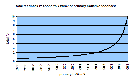
If you are not careful and push the limit, something odd is going to happen. First of all total feedback is growing towards infinity eventually resulting in a division by zero. Even beyond that the feedback returns from the dead, but this time it will be extremely high, and negative, like in the chart below. All of that has no equivalent in reality, or climate respectively.
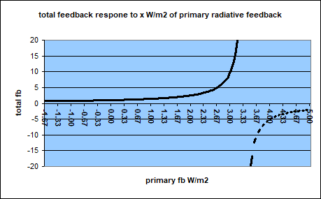
So when dealing with feedbacks you are supposed to keep a safe distance to this twilight zone. If not you might produce a nuclear meltdown like they did in Chernobyl. Or in the case of the IPCC, you run the risk of a) ridiculing yourself and b) cause horrendous damage to the world, by making false “scientific” projections, which they do.
Something interesting happens if we eliminate the negative lapse rate feedback from the above equation. Then ECS will turn into 1.1 / ( 1 – (1.8 + 0.26 + 0.69) x 0.3)) = 6.29K. ECS has grown by a factor 2.4, or alternatively spoken the lapse rate feedback has mitigated total ECS by almost 60%(!), if we compare 2.58K to 6.29K. What the hell is going on?
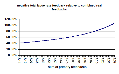
Let us try a systemic approach. Given the named uncertainties, the sum of all three real feedbacks could range from 2.11 to 3.39W/m2, with an average of 2.75W/m2 as above. With a negative “primary LRF” of -0.84W/m2, total LRF would amount to -40.7 to -107.3%(!), with most likely values around -60%. The whole range is far too high, let alone the >100% within the feedback catastrophe. For convenience the chart gives positive percentages btw.
It is a purely logical problem, as with so many instances in “climate science”. Again, lapse rate feedback is technically not a feedback, but the IPCC tries to put all into the same basket. It can not work and it makes absolutely no sense. As a side effect, lapse rate feedback becomes much larger than it could possibly be. Superficially this is ironic, as the IPCC would hardly miss any opportunity to produce as much warming as possible out of any CO2 forcing, while in this instance they seem to give it away for free, by overstating a negative feedback. In reality though, it is a thin line.
Let us test the uncertainty ranges the IPCC names. Then at the upper end ECS excluding lapse rate feedback would be: 1.1 / ( 1 – (1.98 + 0.34 + 1.07) x 0.3) = -64.7K!!! A mitigating lapse rate feedback, like a reduction of 25% to 32%, would do little to keep Earth from falling into deep frost, due to global warming?! The IPCC’s figures are very much testing the logical, or mathematical limitations. You must NEVER push for a feedback of a 100% or more (where it becomes negative!), since then Earth’s climate would be perfectly unstable, which is obviously not supported by reality. The IPCC failed to consider total feedback excluding erroneous “lapse rate feedback” must not violate this logical restriction. And that is even more true, if we consider so called “tipping points”. Since they are not included in these feedback parameters, they would additionally destabilize climate, making it even more prone to a “feedback catastrophe”.
Oops, they did it again!
Driven by a desire to boast high climate sensitivity, the IPCC has overstepped the line. The parameters it uses are depending on a moderating LRF to keep it within the logical limitations. This however, since it is not a true feedback, is a violation of logic on its own right and produces the side effect of an exaggerated and hyperinflated LRF. All this went horribly wrong and you really need to be utmost incompetent to produce such garbage. It may be hard to imagine, but the IPCC delivers, again.
Maybe in a response to this failure the LRF has shrunk to a mere 0.5W/m2 in the latest AR65. However merely reducing LRF is no remedy to the underlying problem. Given a lambda of 0.3 the sum of all feedbacks must not exceed 3.33, yet the IPCC can not help but to notoriously test the limit. In Table 7.10 they give the following intervals. Note: AR6 introduces a new feedback called “Biogeophysical and non-CO2 biochemical”, which is expected to do nothing (central estimate -0.01), but adds a lot of uncertainty (-0.27 to 0.25).
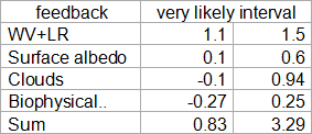
Unsurprisingly the parameters are chosen so that their sum will stay just below 3.33 on the high end, to save it from the “feedback catastrophe”. Yet it comes close with a maximum ECS of 1.1 x 1 / ( 1 – 3.29 x 0.3) = 77K. As before this includes a wrong LRF of -0.5W/m2 and if we pull it out, as we have to, WV feedback will grow up to 2.0 and total real feedbacks up to 3.79, deeply into the twilight zone. And so the whole thing blows up again. From this perspective it seems understandable the IPCC will not endorse nuclear power to fight “climate change”. With this intellect, if they were to operate a nuclear power plant, it would certainly end in disaster.
And still LFR is way too large. The central feedback estimates amount to 2.06W/m2 (= 1.3 + 0.35 + 0.42 – 0.01) with LFR, and 2.56W/m2 without, resulting in ECSs of 2.88K and 4.74K respectively. It is a difference of 39%, well above reasonable estimates of 25 to 32%.
Climate Scientists fail to find the hot spot of mother Earth
Finally there is the issue of theory vs. reality in the way that LRF has been overstated anyway. A part of it is the “missing hot spot” discussion, which is pretty odd. Critics use it to argue climate models would not work, while some proponents of the orthodoxy either deny the mismatch, or claim the hot spot has eventually been found. Thank god we can skip the discussion, as the IPCC openly admits it.
Since 1979, globally averaged modelled trends in tropospheric lapse rates are consistent with those observed. However, this is not the case in the tropics, where most models have more warming aloft than at the surface while most observational estimates show more warming at the surface than in the troposphere (Karl et al., 2006)
A systematic intercomparison between radiosonde-based (Radiosonde Atmospheric Temperature Products for Assessing Climate (RATPAC); Free et al., 2005, and Hadley Centre Atmospheric Temperature (HadAT), Thorne et al., 2005) and satellite-based (RSS, UAH) observational estimates of tropical lapse rate trends with those simulated by 19 MMD models shows that on monthly and annual time scales, variations in temperature at the surface are amplified aloft in both models and observations by consistent amounts (Santer et al., 2005; Karl et al., 2006). It is only on longer time scales that disagreement between modelled and observed lapse rates arises (Hegerl and Wallace, 2002), that is, on the time scales over which discrepancies would arise from inhomogeneities in the observational record.6
The way models work it is certain the LRF has been downgraded over time, without theoretical foundation. Models get parameterized to fit the past, even if the disagreement between theory and observation can not be explained. Without question such an approach is horribly bad “science”, though it happens anyway. And indeed we see a downward trend in LRF estimates over the different IPCC reports, as far they even give numbers. However, as the IPCC is unable to accurately account for LRF, these figures are use- and meaningless, not allowing further analysis, or critique. That is apart from the justified blame of utter incompetence.
For this reason, and because the article is long enough anyhow and needs to come to an end, I will save the discussion on why the “hot spot” is missing for another day. It can only be understood in a wider context anyhow.
Summary:
Lapse rate feedback is technically not a feedback and must not be mixed up with other (true) feedbacks. The IPCC has not learned yet how to account for it properly. Due to this mistake it is impossible to tell what magnitude IPCC suggests for the LRF, as the result depends on the magnitude of real feedbacks, which are subject to wide ranges of uncertainty. Within these uncertainty ranges the IPCC suggests parameters that violate physical, logical and mathematical restrictions. This fact alone outlines (with extremely high confidence) total dilettantism by the “scientists” working with the IPCC.
LRF itself must be seen as a delta in temperature between the effective emission temperature (as a proxy for emission altitude) and surface temperature. Technically this is not a (negative-) feedback, but rather a discount of about 25-32%. Much higher estimates, as suggested in the AR4 for instance (~60%), can not be considered, since they did not know what they were doing, and still do not as with the AR6.
Even though it seems obvious that LRF estimates have been reduced in the face of a disagreement between theory and observation, there are no objections to it. Unintendedly “climate science” produced off-chart high LRF estimates, so that they had to be lowered anyhow. The problem is that this disagreement is a valid hint towards the real cause of the present 5 decadal warming trend, which should have been analyzed, rather than “parameterized”.
Comments (0)
No comments found!