

The Climate Kill Switch – Why Feedbacks are Actually Negative
Outrageous claims may lead to extreme insights. It is as old as epistemology itself and a highly useful tool when analyzing things, I used it many times before. If you think there is a relation, a physical law or something, think it to the ends. What would it mean in the extremes? Is it still plausible then? You always need to put your own thoughts to the test and to anyone mentally fit, this is common procedure.
The huge Climate Sensitivity of > 7K
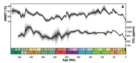
As anyone I am not endlessly creative when it comes to generating own thoughts. That is where outside input, education in the best sense, comes in handy. Let me be straight, without stimuli, the greatest intellects would succumb to idiocy, and that is why Zeke Hausfather’s recent article1 was so inspiring. It claims, with reference to Judd et al 20242, all climate variations over the past 500 million years were essentially driven by CO2. As in the chart below there would be great correlation between CO2 levels in paleoclimate.
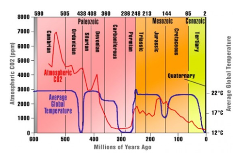
I just want to note there is another “version” of this relation circulating3, arguing the opposite, that there was no correlation between CO2 and paleoclimate. Since I have no crystal ball and am not into the reconstruction of such data, I will have to leave that contradiction uncommented. Some say so, some say so..
The Judd24 chart is interesting in the way that it reaffirms a major talking point of the “critical side”, namely very low temperatures over the last millions of years. In a situation with unprecedented low temperatures and CO2, the rise of both variables does not appear alarming, no matter how you put it.
While Earth has experienced warmer periods in its deep past, the seriousness of climate change is defined by its pace. The warm temperatures in Earth’s past unfolded over millions of years, giving life ample time to evolve. In contrast, today's changes are happening at an unprecedented rate—within decades rather than millennia—leaving inadequate time for adaptation.
Also this argument has little substance. For one this confuses the lack of data as evidence for inexistence. Such reconstructions obviously do not provide the resolution of modern day temperature records. Climate changes of 1-2K (or more) over a few decades are likely not a rare occurrence in the history of Earth. But if the resolution of a climate reconstruction is no better than intervals of 5 million years, it will definitely be blind to such events. For the other we do not have much warming, yet. The “unprecedented rate” of enormous warming is mainly a projection, not a fact. But hey, whatever.
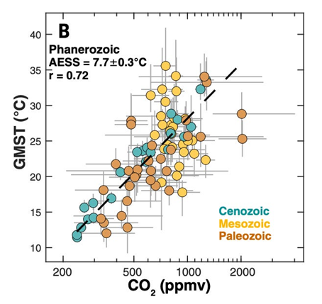
The interesting and inspiring part is something else, the suggested climate sensitivity to CO2. Just to clarify this, we are not talking about ECS in this context. ECS excludes all the long term climate feedbacks, like melting polar caps for instance. This is something not happening over 100, 200 years. At the current rate Greenland would take over 10,000 years to melt, but over the course of millions of years, anything that can happen feedback wise, will also happen. Judd24 assumes an “AESS” of 7.7K per doubling of CO2. Btw. ESS stands for Earth System Sensitivity, AESS may add an Average to it, but I am not sure.
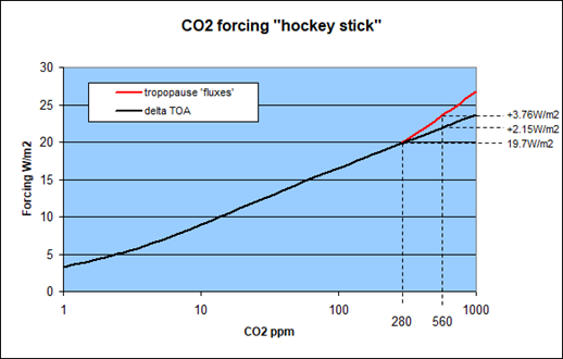
Now let us imagine a world with 2000ppm of CO2 and an average surface temperature of 36°C, as the chart suggests. In the consensus science world a 2,000ppm of CO2 would mean a forcing of 10.5W/m2 (=ln(2000/280)*5.35). Of course this forcing is based on the “flux” approach, while the stock prevailing CO2 is otherwise “forcing” TOA, which leads us to the delicate problem illustrated below. The delta TOA would amount to only 6W/m2.
The issue here is linearity and consistency. The (additional) CO2 forcing due to an increase of it, is just an enhancement of the forcing by the given CO2 amount. So it has to be the same thing following the same rules, obviously. And despite this being crystal clear, “climate science” deplorably fails to account for it.
CO2 forcing & CO2 forcing
Anyway, the point I want to make is, the relation between stock CO2 forcing and enhanced CO2 forcing is pretty stable, regardless of the definition of CO2 forcing. For the sake of argument let me provide this little table below. All the figures were taken from modtran, based on the std atmosphere scenario. The only exception is the canonical 3.7W/m2 forcing under the “flux” concept, which also incorporates assumptions on the changes in stratospheric lapse rates and can not really be reproduced in modtran. Without this factor you get about 4W/m2 in modtran for this approach, which should shrink a little once allowing for it, so that the 3.7W/m2 look quite plausible anyway.
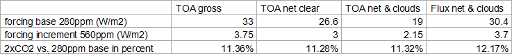
For all TOA approaches the forcing increment is between 11 and 11.5 percentage points for a doubling of CO2, relative to a 280ppm base scenario. Only the “flux” approach yields a something stronger response, like 12.2%, which is not much of a difference either. It looks like “back radiation” from the stratosphere scales just a little better in general, as opposed to the attenuation of upwelling radiation otherwise.
Going from 280ppm to 2000ppm CO2 forcing will increase by ln(2000/280)/ln(2) = 2.84times those respective percentage points. That is from 100% to 132% with the TOA approaches and up to 135% with the “flux” approach. In other words, at 2000ppm CO2 forcing is about one third larger than with only 280ppm. And that is one very interesting perspective.
Let’s be subversive
The one thing not considered here are changes in the lapse rate of the troposphere. First you have the forcing and only then the feedback comes in, be it positive or negative. The forcing rules the feedback, not vice verse, because why would it? And if it did, that would make a horrible mess. And I would assume no one thinks in such perverted ways. But at that point, I just could not help. This was a little obscene eureka moment, not just because it gave me a different perspective on “climate science”, but on my own (published) views as well.
Let us remember that good old emagram4, and what it tells us. While the moist adiabat there is not perfectly in line with some observed (or rather estimated) 6.5K/km at some 15°C, with an atmosphere not perfectly moist either, it provides us with a very good idea on how the lapse is going to change with a different climate. For instance increasing Ts from 15°C to 35°C the lapse rate goes from 5.9 to 3.3K/km, a 44% reduction.
However, the atmosphere will expand if it gets warmer (or vice verse), and so the effective emission altitude would rise even without any addition of GHGs. To allow for this it is way more sensible to relate changes in the lapse rate to a respective pressure level. In that case the delta temperature between surface and 50kPa is 31.2K at 15°C, and 19.45K at 35°C. Although somewhat less than the 44% named before, it is still a substantial reduction of almost 38% (= 1 - 19.45 / 31.2).
CO2 forcing as a whole depends on the lapse rate. If the atmosphere was isothermic, it would arguably not even exist, or be zero respectively. Or in general, if the lapse rate shrinks, so will CO2 forcing, and that is not just true for the increment, but the total. And no, I am not going to explain the GHE again at this point. To cut things short and describe the basic issue: If CO2 forcing increased to a 132% by going from 280ppm to 2000ppm and that leads to a temperature increase of say 20K, this would reduce the lapse rate by 38%, and thus equally reduce the CO2 forcing by 38%. And if you take away 38% of 132%, you get 82%. In other words, because of the enormous heat a 2000ppm of CO2 would generate, due to feedbacks, the total CO2 forcing would then be smaller than it was originally at 280ppm.
Now that is a pretty funny twist, if you ask me. There is no fantasy involved here, but just about filling the gaps in Hausfather’s reasoning (or Judd24 respectively), and adding up the numbers. If Earth System Sensitivity was indeed something of a 7K+ magnitude, you will always run into the fundamental problem of the heating negating the forcing, due to the changing lapse rate.
This will also be true for the “flux” concept, you can find more details on this here. Of the 3.7W/m2 CO2 forcing, about 2.4 come from less upwelling radiation, and 1.3 from additional “back radiation”. Arguably “back radiation” from the stratosphere is insensitive to changes in the tropospheric lapse rate. As in the table above, the “flux” concept would start at 30.4W/m2 CO2 forcing at 280ppm. This would grow by 10.5W/m2 to a total of 40.9W/m2 at 2000ppm. Of these 26.3W/m2 would come from (less) upwelling radiation, susceptible to the lapse rate shrink, reducing the upwelling forcing by 26.3 * 38% = 10W/m2, almost as much as the 10.5W/m2 or original forcing increment. Though, I named 20K of ESS for a 280/2000ppm relation, which equates to only 7K for a doubling of CO2. With 7.7K per doubling, like suggested by Judd24, it would more than cancel out. And there are suggestions of an even higher ESS, like 10K or so, by Hansen5 for instance.
“Equilibrium global warming for today’s GHG amount is 10°C” – Note: Total anthropogenic GHG forcing (not just CO2) today is roughly on par with the forcing assumed for a doubling of CO2 alone.
We end up with an intriguing concept, the representatives of such high ESS values are most certainly not aware of. The CO2 forcing that is supposed to push the climate upward, will get lost on the way up. Per se this idea is not so absurd, we know a lot of analogies to it. If you want to dispose something (like a banana peel in the class room), you can pick it up, carry it over to the bin and put it in. Or alternatively you could stay seated and throw it into the bin over some distance, like the cool kids do – if you have decent aim. In the latter instance you provide the initial momentum and let physics do the rest.
Likewise the CO2 forcing would only provide the thrust to propel the climate of Earth to a different level, but then falls back to the original forcing, more or less, despite a very different concentration. What you get is a scheme like in the graph below, and it is still a defensible concept.
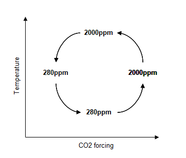
Now this would also work in reverse. If the Earth was a hot house at some 35°C surface temperature and CO2 concentration fell to a mere 280ppm, then the low CO2 concentration and the minimal lapse rate would work together to produce an absolute minimum of CO2 forcing. This might push the climate downward into an ice age.
While I exemplarily picked the extremes of 280 and 2000ppm here, the same relation and cycle would work with any CO2 concentration. The difference would just be about the magnitude of the cycle, or the stretch of time. As long as the time frame is long enough to deploy the bulk of all thinkable feedbacks and ESS is to materialize, it will not make any fundamental difference. The crucial issues here are just the magnitude of ESS and the type of assumed CO2 forcing (TOA or “flux”).
It is far fetched, barely credible, it is not being communicated and most probably not even known in “consensus science”. Yet it is the necessary logical consequence of any ESS in the named magnitudes, and it is still plausible. One could argue this. Also I see how this cyclical CO2 forcing mechanism might be highly attractive and tempting. If there was an innate cycle to it, it is way too hard to not project this on the known issue of ice-age cycles, in some way or another. Just look up Plass 19566. Of course it would not work, because we know temperature leads CO2 over Quartenary cycles.
We have a far bigger issue
First a Recapitulation
At this point I realized I messed up and we are dealing with a much bigger issue then I had realized so far. In “Vapor Feedback II: The Lapse Rate and the Feedback Catastrophe” I discussed a lot of the issues that come along with feedbacks, especially WV and the lapse rate issue. Of course I took a closer look at the emagram, analyzed how the lapse rate would rotate with changing temperatures and how that would affect the whole feedback process.
I was guided by the (correct) idea that CO2 would elevate the emission altitude, and so would WV feedback. The elevation of the emission altitude would a) represent the bulk of climate sensitivity and b) could be translated into a temperature increase at the given average emission altitude, as this should only introduce a minor error margin. The resulting temperature change up there however would be larger than that of the surface, because the rotation of the lapse rate. Bloody simple, so far.
What I derived from all this, was a delta of about 50%. At emission altitude the temperature would increase about 50% more than at the surface, just because of the rotating lapse rate. If all the climate sensitivity was about that emission altitude, we should simply discount it by 33% (=1.5/1) to get the proper value for the surface temperature. Given there are other feedbacks, like cloud- or surface albedo feedback, which are not related to emission altitude, I was quite willing to accept a lower figure for that discount, like 25% only.
Central estimates for LRF (lapse rate feedback) were -0.84W/m2 in AR4, and are -0.5W/m2 since AR5. I had a number of problems with this. The one thing is, if you mix this with other (positive) feedbacks, it dampens the feedback loop, thereby having a highly variable total impact. And LRF of -0.84 would thus reduce ECS by typically 60%, but it could be 80 or even 90% with overall large feedback figures. Despite arguable uncertainty, the ratio between atmospheric and surface warming should be fixed.
For instance with a Lambda = 0.3 (=1/Planck Feedback), a CO2 forcing of 3.7W/m2, positive feedbacks of 3W/m2 and a LRF of -0.84, you get very conventional ECS:
3.7 * 0.3 / (1 – 0.3 * ( 3 - 0.84 )) = 3.15K
Without the negative LRF however, the loop breaks lose so to say..
3.7 * 0.3 / (1 – 0.3 * ( 3 )) = 11.1K
The other problem was the effective magnitude of LRF. It just would not make sense to assume the troposphere would warm like 3, 4 times as much as the surface, or even more. According to the emagram above it could be up 1.6imes as much, but nothing more. I interpreted the sharp drop in LRF from AR4 to AR5 as a lukewarm “hot fix” to this problem, yet still overstating (negative!) LRF.
Eventually primary feedbacks must not exceed 1, because that would mean a perfectly unstable system, prone to tip over one or another direction at any time. Since I considered LRF not a real feedback, but just the difference in warming between mid troposphere and surface, I agued this condition must be met excluding the negative LRF.
Here is my dear mistake
I only projected the LRF on feedbacks themselves, and as far as that goes I stand to all I said. However, I should also have projected it on CO2 forcing itself, and not just the increment, as discussed above. But it will not end there. The whole of the GHE is affected by it. It is a very simple relation, if the lapse rate shrinks by 1%, the GHE shrinks by 1%. And if the lapse rate was zero, meaning the atmosphere was isothermic, there would be no GHE.
Psychologically speaking, I was taking a step back get a better perspective, but that was a few steps short of what I should have done. I tend to criticize people for being too narrow minded, only thinking within their box of reference while avoiding the full width of available perspectives. What can I say, it also happens to me.
No Lapse Rate, No GHE
Let me add an external source on this issue, let me quote Brian E.J. Rose7, a climate expert from the University of Albany. I know there are many other sources, but I am lazy and I just do not mind looking them up.
Greenhouse effect for an isothermal atmosphere
Stop and think about this question: If the surface and atmosphere are all at the same temperature, does the OLR go up or down when € increases (i.e. we add more absorbers)?
Understanding this question is key to understanding how the greenhouse effect works.
Let’s solve the isothermal case. We will just set Ts = T0 = T1 in the above expression for the radiative forcing.
What do you get? The answer is R = 0
For an isothermal atmosphere, there is no change in OLR when we add extra greenhouse absorbers. Hence, no radiative forcing and no greenhouse effect. Why? The level of emission still must go up. But since the temperature at the upper level is the same as everywhere else, the emissions are exactly the same.
The radiative forcing (change in OLR) depends on the lapse rate!
Yes, of course! Let me go back to my simple but accurate depiction of the GHE. It is nothing special, you could also get this from Held, Soden 20008. I think it is, and has always been, evident how the tropospheric lapse rate is essential to the very existence of the GHE. No lapse rate, or rather a lapse rate of zero, no GHE.
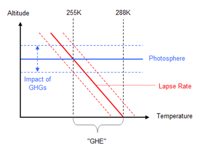
For the sake of argument let illustrate what happens if the lapse rate gets lost, or at least partially lost. Per se it is not the emission temperature, or the emission altitude that changes, but the surface temperature. The first two are both fixed due to a) the energy budget, that is the amount of solar energy being put into the system, and b) the concentration of GH-agents within the atmosphere.
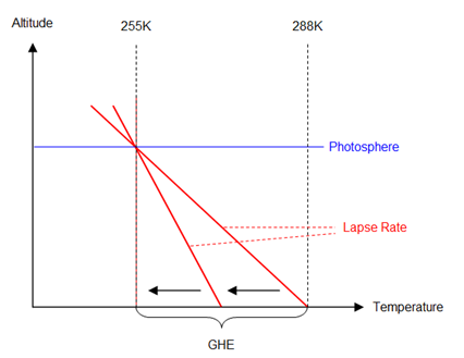
It is an isolated view just on the lapse rate. There is nothing going on with the emission temperature, or the altitude of the photosphere, all that remains the same. What is actually changing is of the course the lapse rate and with it a) surface temperature and b) the magnitude of the GHE. Again, this is crucial to understand. In an isothermic atmosphere, the emission temperature equates to the surface temperature and because the emission temperature is fixed, as the energy budget is fixed, the surface temperature drops to exactly this low value.
While an isothermic atmosphere with a lapse rate of zero is just a theoretic consideration, a reduction of the lapse rate is not. The only question is by how much. I took a very close look at the emagram and based on the temperatures of surface and 50kPa, I typed all the data into an excel sheet. Given there are only lines and thus intersections for every 5K in surface temperature, I opted for intervals to represent the specific slope. It goes like what happens between 10°C and 15°C in surface temperature, then between 15°C and 20°C, and so on, with the average of the interval given at the x-axis.
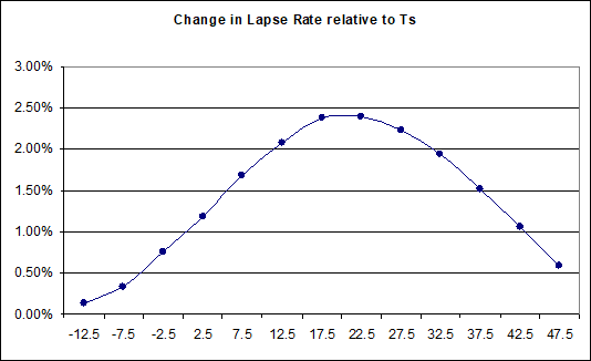
If the chart does not look perfectly smooth, it is because I had to read the data from the chart, so to say “between the lines”, quite literally. I can not say the emagram as such is correct, but I understand it is well established in meteorology, an actual science. And if it is true, it tells us how the lapse rate is supposed to change with a variation surface temperature. Despite the percentage figures being positive here, they actually mean a reduction in the lapse rate going from left to right (meaning warming), or an increment going the opposite way (meaning cooling).
Why this distinct shape?
Why would it go this way? I can only guess. With low temperatures the latent heat issue vanishes. There will barely be evaporation at the oceanic surface, then there is not much to condensate and the impact of WV on the lapse rate becomes negligible. With high temperatures on the other end, the limits might be harder to push. With a surface temperature of 50°C the 50kPa level is at 33.5°C, only 16.5K difference, or 2.6K/km. Maybe that is a level that is just hard to push further, especially so if it still contains an “unstable component” due to convection, which should be unaffected by temperature. Anyhow, I have no expertise on this and so I will just stick with the data as they are.
Is the same theory also used in “Climate Science”?
Another necessary consideration is on whether the emagram is even representing the bigger picture, in the sense of is this consistent with a change in global climate. I mean maybe it is just weather, or something. That is where Santer et al 20059 comes handy. Among the co-authors are G. Schmidt, G.S. Jones or J.E. Hansen, not very alternative science so to say. They provide the chart below on the tropical lapse rate trend, with the thick black line named “theory”. The colored lines are model outputs and the two lines to the left are empirical evidence, and yes there are some issues going on. But that is not the point here.
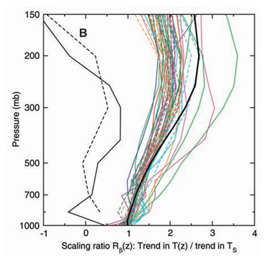
Rather that “theory” is perfectly consistent with the emagram. In the emagram the 300mb pressure level warms 2.3 to 2.5 times as much as the surface with tropical temperatures, in this chart it is about 2.35K vs. 0.95K, spot on. So that tells us we are talking about the same theory and the emagram is indeed the theoretical foundation.
Btw. the fact that models, on average, have a lesser change in lapse rate than the theory, should not surprise. This is the warming over the whole of the tropics and there, as anywhere else, land is warming faster than the ocean. With the ocean, or SST lagging behind, the same should be true for WV concentration and LRF. It will not mean a fundamental disagreement between theory and models.
The Mission Implausible
And here is the real problem, outlined in the graph below. If the lapse rate shrinks by 2.1%, which is roughly the “theory” at current average global temperatures, you inevitably get this result. Everything else being equal, the emission temperature (Te) will grow by 1.7K for every K warming of Ts. Holding on to a simple blackbody assumption, emissions increment by 6.5W/m2, 3.2W/m2 more than a “Planck Feedback” of 3.3W/m2, meaning an LRF of -3.2W/m2.
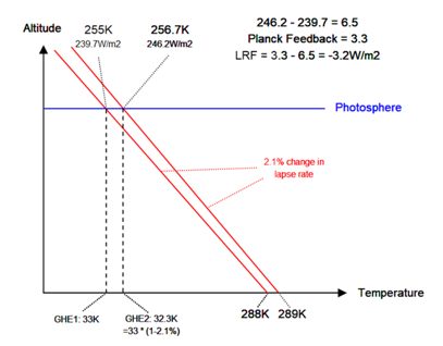
That is a negative feedback of 3.2W/m2, easily exceeding all thinkable positive feedbacks. In other words, this alone negates basically everything “climate science” stands for. The official LRF is at -0.5W/m2, consistent with a mere 0.3% change in the lapse rate. We are talking about different dimensions here, pivotal to the whole subject of “climate change”. It is an unforgiving “detail” and I tried my best to consolidate it.
The Exploration
I went through a number of papers, searched all IPCC assessment reports from AR2 upward, but there was nothing tangible. There is not much talk on the lapse rate in the first place, AR2 for instance mentions it 9times, remaining superficial and avoiding the core issue. And it stays like that, up to AR6. Why the lapse would change according to the “theory” as in the emagram, but LRF on the other would be much lower, remained a mystery.
So I turned to AI (ChatGPT, Grok, DeepSeek) and tried to get some answers there. I know AI is no good when it comes to logical reasoning, or mathematics, because it just imitates. But effectively it is also a search engine and so it should be able to provide answers, if it can find them. Soon I realized a certain pattern. I would come up with the basic problem, how a change, or reduction respectively, of the lapse rate would necessarily need to cause LRF, and how this was inconsistent with “consensus science” figures on LRF. The AI would always spin the problem in a way to come up with the consensus position in the end, and violate all logical restrictions on the way.
For instance it would agree that LRF must be large, like -3W/m2 or so, in theory, but that would attenuated by WV feedback. I would respond this was pointless, because these are separate entities. Then it would simply suggest an incorrect calculation to get over the issue. Pointing that out, it suggested to reduce the consolidated LRF/WVF by WVF a second time, just to get to a positive feedback all over. Over many iterations, with different AI engines, I remained stuck in Groundhog Day. For instance I also got this claim:
Net result: ΔT_e = 1.2–1.5 K, with a positive combined feedback.
Grok here claims that the emission temperature would increase more than the surface temperature (per 1K Ts), and this would indicate a positive(!) feedback. We had talked about this before and so this is not just factually wrong, but Grok also knew already that emission temperature increasing more than surface temperature was a negative feedback, and vice verse. And at this point I realized the problem.
I was asking a question for which there was no answer, at least none that could be found online. The AI only knows the final result, which is the consensus position of a minimal LRF (-0.5W/m2) and a positive combined feedback, but has no clue how to get there. Just like myself, it could not find a consistent source on this, and so it is just making it up, breaking the rules of logic every single time. No matter how many times I would correct the AI on its blunders, it would reiterate and introduce new ones, or bring back older ones. Frustrating and useless!
The Solution, finally
At this point I was kind of giving up. I understood the science is wrong on the most fundamental issue of LRF, and that it is the only reason why total feedbacks are positive, rather than negative. But I could not find HOW it was wrong. And that is when I ran into a crazy, unbelievable “conspiracy theory”:
Feedback parameters in climate models are calculated assuming that they are independent of each other, except for a well-known co-dependency between the water vapour (WV) and lapse rate (LR) feedbacks
If this was true, it would mean the lapse rate would not determine LRF, but rather that it be fixed in advance, so that the LRF is always smaller than the WVF, by about 1W/m2, no matter what. It is like fixing a football game where you determine team A will win by 2 goals over B, regardless of what happens on the field. It could be 2:0, 3:1, 4:2 and so on, but nothing else. Of course that would address our problem over why the rotation in the lapse rate, like in the emagram or S05, does not produce an accordingly strong LRF in the models, as it should. It is just not allowed to, despite physical necessity.
So who is making this unfathomable accusation? It is the IPCC in AR6, WG1, page 978!!! Facepalm! In this way they can rotate the lapse rate in the models, without causing the according negative LRF. And this is not just an evident violation of physics, but a political necessity, so to say. Otherwise a huge negative LRF would have to dominate all the positive feedbacks carefully constructed. You have to break the rules, you have to deny simple physics, if you want to support the “consensus science” narrative, and that is apparently what they did.
But it is even worse. We need to consider why “consensus science” is so confident over combined WVF – LRF being positive. It is a) because you need huge amplifiers to argue CO2 being the cause for paleoclimate variations and b) because the observed dOLR/dTs relation is apparently providing evidence for it. The problem is, we know b) is definitely wrong as I have discussed and a) is just an unsubstantiated theory not working.
This is just typical human behaviour, as old as mankind itself. You have a certain perspective, you align with it and consider it true, and from there on you want it to be true. While it is just a perspective, and as such circumstantially true, if at all, people love to declare it to be “the truth”, with all other perspectives contradicting then being a lie. That is what got is religions, ideologies, superstition, dogmas, and of course bad science. Instead of carefully considering all the different perspectives, or bits of - in this case - conflicting information, they “settle the truth” and use brute force against what is not fitting. And in the context of climate models, they just hard-coded the WV-LR feedback relation, instead of allowing LRF to do what is physically opportune.
Summary:
Reconsidering my previous claims, I have to point out lapse rate feedback should indeed be treated as a feedback, and it appears to be massively negative. When the theory, as represented in an emagram and implicitly confirmed by for instance Santer et al 2005, is correctly applied, LRF amounts to about -3W/m2, with a tendency to grow even larger towards -3.5W/m2 over discussed global warming yields (ECS, ESS). The figure significantly exceeds positive feedbacks (central estimate AR6: 2.58W/m2; consisting of 1.8W/m2 WV-, 0.42 cloud-, 0.35 albedo- and -0.01 “geophysical” feedbacks)
As an intriguing and non negligible detail, LRF also has to dampen CO2 forcing itself. Depending on the definition of CO2 forcing, it is going to be between 13 to 20 percent per Kelvin of warming. There are all kinds of implications to this, however to my knowledge, this has never even been considered.
One might expect such a theory of a strong lapse rate rotation and accordingly strong negative lapse rate feedback, would be rejected within “climate science”, and be replaced with something else, as it might jeopardize the whole concept of a climate system rich in positive feedbacks. Notably that seems not to be true. Instead another, very dull “solution” was opted for - by simply hard-coding a positive WV-LR feedback into the models, no matter what, independent of what the lapse rate does, thereby violating logical and physical constraints. This is preposterous, a simple act of cheating. You will not do that erroneously, but rather in full awareness of misconduct.
Theoretically the sum of climate feedbacks should be negative. Practically there is nothing contradicting this notion. What actually stands in the way is the belief of a positive WV-LR feedback, which itself is based on a misperception, as previously discussed.
4en.wikipedia.org/wiki/Emagram – from R.B. Bull “Meteorology for Scientists and Engineers”
9http://www.atmo.arizona.edu/students/courselinks/spring09/atmo656b/Santer_2005_UpperTropWarming.pdf
Comments (9)
radiativeTransfer
at 18.06.2025great article like always.
I played a little bit with Grok, asking for a mathematical example of total feedback (planck + lapse rate) for a simplified atmosphere of two layers, surface and 300hpa, a 1K increase in surface temperature Ts, a 2K increase at Te, a standard Planck feedback of −3.2 W/m2/K.
The result was an integral formula for lapse rate feedback, that in my case, was just the sum of two components, surface and 300hpa. The variables of the formula are KT(z): Radiative kernel and ((∂T(z)∂Ts)-1): Temperature change at level ( z ) per 1 K surface warming.
If you follow the examples, its pretty straight forward, and the result is a lapse rate feedback of -0.8W/m2/K. As far as you read the examples, the core is about the kernel values based on climate model studies (e.g., Soden et al., 2008).
Its difficult to see from where you got the -3.2 W/m2/K of feedback at 300hpa.
Could you explain a little bit the difference between your simplifed model and the standard radiative kernel with a simplified atmosphere?
thanks.
GHD
at 19.06.2025300hpa is pretty high up for an average emission altitude, even in the tropics. But for the sake of argument let us assume it was 255K up there and that T(z) was going up by 2K.
255^4*5.67e-8 = 239.74
257^4*5.67e-8 = 247.35
OLR then would increase by 247.35-239.74 = 7.61W/m2
In other words, you would need a forcing of 7.61W/m2 to increase Ts by 1K. With a 3.2W/m2 forcing you would only get 3.2/7.61 = 0.42K warming. Or you can split up the factors and name it a negative feedback of 7.61 - 3.2 = 4.41W/m2. It then is like..
3.2/3.2 * (1/(1-(-4.41/3.2))) = 0.42K
In words: a 3.2W/m2 forcing would equate to the planck feedback and thus equate to 1K in forcing. Due to a negative feedback of -4.41W/m2 it would only result in 0.42K in surface warming.
All that is inevitably so, yet Grok will "calculate" something very different..
radiativeTransfer
at 20.06.2025i am totally sure the issue is about my interpretation, but i still don't see it. I have uploaded three screenshots of the math involved in calculating the lapse rate feedback for a two layer simplified atmosphere, Ts and 300hpa (around 9km). Its divided in three screenshots. The first one (https://ibb.co/0jYtrVnn) show the general formula for lapse rate feedback. The Radiative Kernel Kt(z) is the relevant variable, because the other component is trivial. In here (https://ibb.co/HDKW8PQ8) we have the Kt(z) for Surface, and in here (https://ibb.co/TqvYnDKR) for 300hpa.
Where is the math error from your point of view? where is the variable that is producing the official LRF of -0.5W/m2 ? Maybe is the whole formula?
Thanks in advance.
GHD
at 21.06.2025The reduction in the lapse rate means Tz (or T300 if you will) will increase MORE than Ts, like Ts+1 and T300+2. Try that..
radiativeTransfer
at 22.06.2025sorry for the delay. I provide you a Grok answer for this basic atmosphere tropical scenario.
https://limewire.com/d/KRmcu#AOiLKyNiIt
GHD
at 23.06.2025AND the AI makes a lot of calculating mistakes, sometimes small, sometimes large, but always on purpose. For instance 230^4*5.67e-8 = 158.67 and NOT 158.96! This difference of 0.29 eventually shrinks the lapse rate feedback in this calculation.
radiativeTransfer
at 23.06.2025totally right, Grok is a fountain of errors. You have to be really carefull following all the reasoning, because the initial setup conditions could be changed during the real time calculations. I didn't expect this behaviour.
I try another approach, setting Ts (surface temperature) for a 1K warming generating and Tut (upper troposphere temperature) feedback of 1.7K.
https://limewire.com/d/ghx3Y#LcMDHP47Me
Give me your thoughts if possible to, at least, stablish a common ground
GHD
at 23.06.2025(390.06 / 2) / 314.8 = 62%
With your model it is still 62%. The bulk of your OLR thus is totally insensitive to changes in the lapse rate, thereby undererstimating LR feedback.
Btw.. if you want to discuss this further, do it by email. Your email address however does not look legit.
Christopher Game
at 01.08.2025