Why 2W/m2 CO2 forcing is actually quite certain
It is funny how the content of this largely ignored site sometimes diffuses into the world. Of course such education is its scope, but one might expect people to communicate a little more open on what their source is, or ask for clarification if the content is too complex for them. After all this would help to spread the word and gain me some well deserved reputation.
Bob Irvine’s misunderstanding
Just a few days ago I had a little déjà-vu while reading an article on WUWT. The title was “The Climate Feedback Debate”1, sounding interesting to me. After a couple of paraphrases I could not help but to realize I read it before. That was when I was check-reading my own article “Vapor Feedback II: The Lapse Rate and the Feedback Catastrophe”. Bob Irvine changed a few things there and there, added some charts on the development of atmospheric WV concentration, but otherwise stayed close to the original. That is without referencing it, except under one adapted chart.
The other problem, those changes were largely not for the better. Not explaining the lapse rate feedback (LRF) is one thing, although I guess most readers there would benefit a lot from such understanding. Adding wrong assumptions is yet worse. The central estimate for bio (-geophysical and –chemical) feedback introduced with AR6 is not -0.1, but only -0.01. Notably these central estimates on feedbacks are not quite sufficient to support an ECS of 3K. With a (2xCO2 forcing) of 1.1K it is only 2.58K in AR4 and 2.88K in AR6. This led him to believe there would be further, unnamed feedbacks.
This is wrong. In reality, because of the feedback loop, ECS projections are of a logarithmic scale. Considering the uncertainties, deviations from central estimates will be small towards lower, but large towards higher outcomes. For instance, if the central estimate for ECS was indeed 3K, then mathematically a 2K result is about equally likely as 6K(!). Let us say total feedback was 2.11W/m2, +/- 0.61. Then..
1.1 / (1 – 0.3 * 2.11) = 3K
1.1 / (1 – 0.3 * (2.11 - 0.61)) = 2K
1.1 / (1 – 0.3 * (2.11 + 0.61)) = 6K
If you only hear about an interval of 1.5K to 4.5K, with 3K as central estimate, you will tend to assume a linear scale, but that is not so. These are simplified figures optimized for communication. So again, this outlines the problem with the discussion on the “critical side”. People do not understand, but assume instead, and their assumptions tend to be wrong. But I digress..
Wijngaarden’s uncertainty problem
What I actually wanted to talk about is way more significant. As you may know Wijngaarden and Happer are trying to solve the riddle how clouds would influence CO2 forcing. As absurd as it is, spectral line calculations, on which these estimates ARE based on, have never included clouds. Moreover they have not even allowed for overlaps between the different GHGs. So we are talking about the most basic climate research one could only imagine, and it has never been done.
Never?`Well of course I did it recently, and Ollila2 made an attempt. Otherwise there is nothing, to my knowledge. Now Wijngaarden recently starred on Tom Nelson’s podcast, where he outlined that under certain conditions, high up clouds (from tropical thunderstorms rather than cirrus) could even mean a negative CO2 forcing. This again triggered Nelson, who wanted to learn more about it. Of course, if you hear that for the first time, you might think maybe this is the key to falsifying the AGW theory, which it is anyhow. It is just not that simple. Anyway, here is Wijngaarden’s response.3
“This calculation would show a negative forcing, if we double CO2, was for clouds in the western pacific at this altitude of 11 to 13km. For other clouds at different altitudes you do not get cooling. So the point here is not to say clouds overall cause forcing to go negative. Overall they are probably going to cause the forcing to be less positive. I think the consensus view, even when you talk about to people in the global warming community, is that a forcing for clear skies of CO2 which is about 3W/m2. When you take clouds into account, it is going to reduce it about 30% to about 2W/m2. But that is where there is a lot of uncertainty at the present time, figuring out what is going on with clouds.”
Now that sounds pretty familiar, considering my own work. I would not know who else has ever pointed out 2xCO2 forcing to be actually just 2W/m2. Although that is not just because of the consideration of clouds, but also includes the deviation of real surface emissivity vs. from model assumptions. It would seem the “consensus view” in the “global warming community” is pretty much my own disruptive work.

Now the point I would like to take on, is the claim there was a lot of uncertainty about it. As it goes what I write and publish is pretty profound. I see little reason to only scratch at the surface and want to take things further. Yet, as with any onion, there are even deeper layers which I use to sure up the perspectives presented. Just like in chess you want to think a few moves ahead. In no way it means perfection, but it helps to sort out a number of mistakes, misperceptions that could occur otherwise.
In the given context it means I did not just assume some random cloud models provided by modtran, very simplified indeed, but at least interpolated, would provide enough secure evidence to quantify their effect on CO2 forcing. Rather there was another layer behind it I did neither publish nor discuss. So let us do it now. But first let me show you the chart Wijngaarden presented.
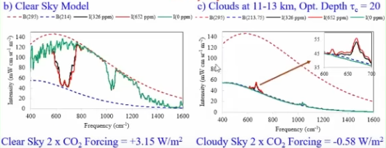
This is a tropical scenario in the western pacific. I do not know the exact parameters here, like latitude or temperature, but obviously with a warmer than average climate CO2 forcing will be larger. Also the tropopause there is relatively colder than with a typical standard atmosphere. Now what he did here is to simply introduce an opaque layer at the given altitude and so all the emissions from below become irrelevant for total outgoing emissions. Rather in this scenario, all that matters for outgoing emissions is the cloud layer and its (low) temperature itself, and the few GHGs above this layer.
Above the tropopause comes the stratosphere where temperatures increase with altitude. When you double CO2 the emission altitude increases and, holding everything else fixed, the emission temperature increases and emissions with it. Because of it then CO2 forcing will be negative. So yes, under these circumstances with altitude clouds, the inclusion of these clouds can reverse the otherwise warming effect of CO2.
Yet, although I have (re-)produced this perspective before, there is a lot of trouble with it. First of all this is under the assumption the atmospheric temperature profile was fixed, which it is not. Rather when you increase CO2 the stratosphere will cool and that minimizes the negative CO2 forcing in this instance. Second and more profoundly, it suggests there was a wide range of possible outcomes for cloud integrated CO2 forcing. That just leads us, or him respectively, onto the wrong path, while an accurate solution was right at his finger tips.
Digging into the data
Here is the procedure. I took the “raw model output” from modtran and transferred it into Excel. With this are no longer restricted to the few options modtran offers, and instead, if you know what you do, you will have a lot more options to process and analyze the data. Doing so for a standard atmosphere model we get the two curves in the chart below. The difference between these two amounts to 2.96W/m2. Remarkably this is a bit less than what you get in modtran (2.983W/m2) and that is probably because these data only reach up to WN 2200. There is still about 0.5% of the emission spectrum left beyond WN 2200, including a smaller absorption band of CO2. Apart from this little issue, the data are fine and otherwise consistent with hitran output.
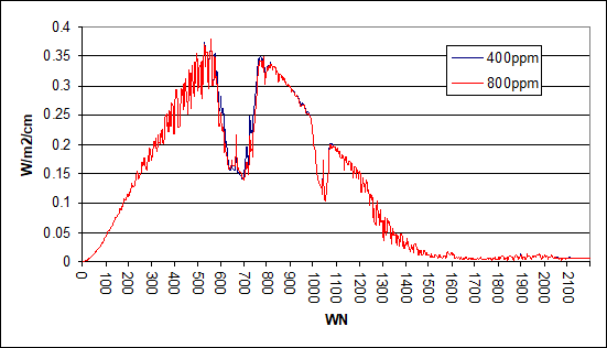
Notably in the chart above the red line is below, or on par with, the blue line, meaning less emissions because of more CO2. But there is an exception from WN 640 to 696, where it is the opposite. In this range CO2 has its highest absorption rate and the emission level is already in the stratosphere. We will account for it separately.
Now the gloves are off and we can do pretty much the same thing Wijngaarden presented in the quoted chart. First we introduce a cloud layer at emission temperature of 220K, meaning it was top of the troposphere. This would also be the coldest temperature in a typical atmospheric profile. The troposphere below is warmer, and so is the stratosphere above.
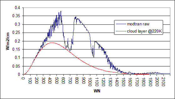
Because of it we can assume all emissions exceeding that of our slab cloud layer will come from underneath it, therefore being covered by the clouds and becoming irrelevant. The exception here would be the stratospheric part of which we know that despite it having higher emission temperatures, it will be above the cloud layer. Doing this we get the result below, which a 2xCO2 forcing of -0.37W/m2. It is a little less than the -0.58W/m2 Wijngaarden names, but keep in mind we have a different data source and most of all a standard atmosphere model, as opposed to the tropical scenario he used.
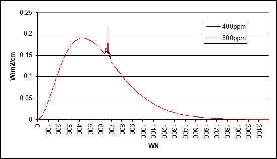
At this point there is an interesting and utmost important detail in the data, which Wijngaarden apparently did not recognize. Not just the 2xCO2 forcing dropped from 2.96W/m2 to -0.37W/m2, but also outgoing emissions are very low. In this model emissions are only 133.43W/m2, and the CRE 134.W/m2. It is an extreme, hyperbolic scenario with little merit if we look at it isolated. But once we look at the relation between the CRE and the reduction in 2xCO2 forcing that is no more so. In this instance outgoing emissions shrank by 50.18% and 2xCO2 forcing by 112.4%. The ratio is 1 to 2.24, and I can already tell you this ratio would not be very different in Wijngaarden’s example.
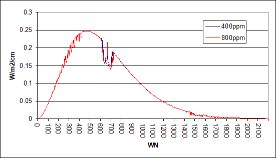
The important question now is, how this ratio holds if we go through different cloud altitudes. For instance we can do the same thing assuming a cloud top temperature of 260K (see below), corresponding to an emission altitude of 4.34km. Then the CRE is 43.93W/m2 and 2xCO2 forcing is at 1.83W/m2. Percentage wise the reductions are 16.4% in total emissions and 38.5% in 2xCO2 forcing. The ratio here is 1 to 2.35.
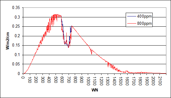
The same with emission temperature of 240K and an inferred altitude of 7.42km..
Of course I went for the systemic approach and did this for all kind of cloud altitudes and temperatures. Below there is shortened table with the results from it. The cloud top altitude here is simply derived from the emission temperature, assuming a lapse rate of 6.5K per km.
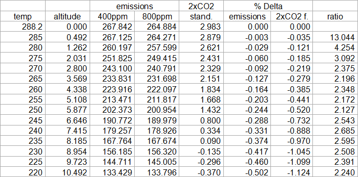
This model is by no means perfect and I have done further iterations hereto. For instance I simply used perfect emissivity for clouds here, while modtran has surface emissivity at 0.975. This falsely produces far too high ratios for low altitude clouds. Also this simplified approach produces somewhat too low ratios at very high altitudes. I could produce a lot more data and go through all the peculiar details and discuss them thoroughly, but I am pretty sure this would hardly be appreciated. Instead I prefer to point into the right direction, provide the right ideas, and if you really want to go for it on your own, you have a star to follow.
Note: there is a pretty constant ratio between CRE and CO2 forcing reduction
Rather we should probably short cut this to the main point. Although it varies a little bit with different altitudes, overall the ratio is about 1 to 2.5 on average. And this insight is all we need. Regardless of how complex clouds are, whether they have low optical depth, at which altitude they emerge, relative to the reduction in outgoing emissions due to the CRE, 2xCO2 will decrease about 2.5times more.
On top of that we have another restriction. We know the CRE must reduce outgoing emissions by about 11%. If clear sky emissions are 267.8W/m2, then including clouds it should be about 267.8 * (1-0.11) = 238.4W/m2. Also a CRE of then 29.4W/m2 is highly consistent with consensus estimates. Thanks to the relative constant ratio of 2.5 we can tell, the reduction of 2xCO2 forcing will be about 27.5% (=11% * 2.5). Once we apply this “discount” on a clear sky 2xCO2 forcing of 2.98W/m2, we get down to 2.16W/m2. It is not exactly 2.15W/m2, but who cares?
So because this ratio shows little variation, we have a leverage. It does not provide ultimate precision, but we can tell with high confidence that the inclusion of clouds will drop 2xCO2 forcing to about 2.15W/m2. It may well be a few hundreds more or less, but relative other uncertainties in climate science, it is really a tight result. Most certainly it will not be beyond a 2.1 to 2.2W/m2 range. And with this knowledge in mind, the simple interpolation of straight forward modtran results I presented was perfectly fine.
So that is that. Nothing new here, just some background information to climate essentials you won’t learn anywhere else. And of course this is just one little detail if we consider the wider context. Ultimately CO2 forcing will be even lower because of the issues with surface emissivity. More importantly the same basic issue applies to other GHGs, most notably water vapor.


Comments (6)
Robert Hendriks
at 06.02.2023Why do you think Wijngaarden & Happer have tried to publish their two recent work papers on three major physics journals, and those three rejected them (and probably will happen with their third paper in progress about clouds)?
https://arxiv.org/abs/2006.03098
https://arxiv.org/abs/2103.16465
Its difficult to trust this kind of reasoning, even when it sounds reasonable, when almost nobody in the mainstream science is backing up with relevant papers published on main journals.
Cheers.
GHD
at 06.02.2023Doug MacKenzie
at 18.02.2023Doug MacKenzie
at 18.02.2023They show in fig 22 that surface would be 20 degrees warmer in clear sky as opposed to cloudy sky. A good argument for us climate rationalists.
https://geosci.uchicago.edu/~archer/warming_papers/manabe.1967.rad_conv_eq.pdf
PS, Hope you haven’t been insulted by a couple of my comments to your comments on WUWT. Your work is commendable.
GHD
at 10.03.2023It is one of the many false friends the "climate rationalists" like to fall for. Manabe himself is probably one of the worst "climate scientists" ever, his work is extremely incompetent. There is insurmountable irony in him getting a nobel prize.
First of all his idea of a "back radiation" induced GHE is not just wrong, it "inspired" generations to come to misunderstand the GHE. Only in AR5 the IPCC eventually dropped "back radiation" from its GHE definition.
Second he elaborated this "back radiation" concept to a multi-layer model. This concept could easily be used as a blue print for a "Manabe-Strickler" device to produce free energy. Not just it would easily solve "climate crisis", but you would have a universal perpetuum mobile. Certainly worth a nobel prize - if it worked. Which of course it does not!!!
Thirdly he totally misunderstood clouds. There are not cooling but warming Earth. If have discussed the logical issues "the science" has with it in detail..
https://greenhousedefect.com/the-beast-under-the-bed-part-1
https://greenhousedefect.com/basic-greenhouse-defects/the-beast-under-the-bed-part-2
..and some empirical data here (I should release more..)
https://greenhousedefect.com/the-cloud-mess-part-2-something-spooky
I know you are hooked on the idea of explaining warming with a reduction in (low) cloud cover. I am afraid that is NOT how it works.
LOL@Klimate Katastrophe Kooks
at 20.03.2024"First of all his idea of a "back radiation" induced GHE is not just wrong, it "inspired" generations to come to misunderstand the GHE."
It can be mathematically and scientifically proven that 'backradiation' is nothing more than a manifestation of the misuse of the Stefan-Boltzmann equation by the climatologists. It not only does not occur, it cannot occur. Energy does not and cannot spontaneously flow up an energy density gradient. The 'backradiation' claim is directly analogous to claiming that water can spontaneously flow uphill (ie: up a pressure gradient).
Most people cannot think in terms of energy, energy density and energy density gradient. We need to analogize to something they’re familiar with. Thus, just as, for instance, water only spontaneously flows down a pressure gradient, energy only spontaneously flows down an energy density gradient. That’s 2LoT in the Clausius Statement sense, in a nutshell. So one tack to take is to ask people if water can ever spontaneously flow uphill. Of course they’ll say, “No, water cannot flow uphill on its own.” Then show them dimensional analysis.
mass (M), length (L), time (T), absolute temperature (K), amount of substance (N), electric charge (Q), luminous intensity (C)
We denote the dimensions like this: [Mx, Lx, Tx, Kx, Nx, Qx, Cx] where x = the number of that dimension
We typically remove the dimensions that are not used.
Force: [M1 L1 T-2] /
Area: [M0 L2 T0] =
Pressure: [M1 L-1 T-2] /
Length: [M0 L1 T0] =
Pressure Gradient: [M1 L-2 T-2]
Explain to them that Pressure is Force / Area, and that Pressure Gradient is Pressure / Length. Remind them that water only spontaneously flows down a pressure gradient (ie: downhill). Then introduce energy. Tell them that energy is much like water. It requires an impetus to flow, just as water requires an impetus (pressure gradient) to flow. In the case of radiative energy, that impetus is a radiation energy density gradient, which is analogous to (and in fact, literally is) a radiation pressure gradient.
Energy: [M1 L2 T−2] /
Volume: [M0 L3 T0] =
Energy Density: [M1 L-1 T-2] /
Length: [M0 L1 T0] =
Energy Density Gradient: [M1 L-2 T-2]
Explain to them that Energy Density is Energy / Volume, and Energy Density Gradient is Energy Density / Length.
Highlight the fact that PRESSURE AND ENERGY DENSITY HAVE THE SAME UNITS.
Also highlight the fact that PRESSURE GRADIENT AND ENERGY DENSITY GRADIENT HAVE THE SAME UNITS.
So we’re talking about the same concept as water only spontaneously flowing down a pressure gradient (ie: downhill) when we talk of energy (of any form) only spontaneously flowing down an energy density gradient. Energy density IS pressure, an energy density gradient IS a pressure gradient… for energy.
It’s a bit more complicated for gases because they can convert that energy density to a change in volume (1 J m-3 = 1 Pa), for constant-pressure processes, which means the unconstrained volume of a gas will change such that its energy density (in J m-3) will tend toward being equal to pressure (in Pa) (see below). This is the underlying mechanism for convection. It should also have clued the climastrologists in to the fact that it is solar insolation and atmospheric pressure which ‘sets’ temperature, not any ‘global warming’ gases.
Since a warmer object will have higher radiation energy density at all wavelengths than a cooler object (because remember, temperature is a measure of radiation energy density, equal to the fourth root of radiation energy density divided by Stefan’s Constant):
https://i.stack.imgur.com/qPJ94.png
… ‘backradiation’ can do nothing to warm the surface because energy cannot spontaneously radiatively flow from lower to higher radiation energy density, and thus CAGW is nothing more than a complex mathematical scam perpetrated to obtain multiple billions of dollars in funding for trough-grubbing line-toeing ‘scientists’ and to push a Marxist One World Government “Build Back Better” agenda.
“But they’ve measured backradiation!”, some may claim. Yeah, no.
https://claesjohnson.blogspot.com/2011/08/how-to-fool-yourself-with-pyrgeometer.html
As Professor Claes Johnson shows in that article on his website, pyrgeometers (the instrument typically used to ‘measure’ backradiation) utilize the same sort of misuse of the S-B equation as the climastrologists use. The bastardized form of the S-B equation used by pyrgeometers [ usually some form of q = (σ Th4 – σ Tc4) or equivalently Ld = Uemf/S + σTb, as outlined in the documentation for the instrument, with Uemf/S being negative in sign ] apriori assumes a subtraction of ‘cooler to warmer’ energy flow from ‘warmer to cooler’ energy flow, which as has been shown above, is fallacious.
https://i.imgur.com/QErszYW.gif
The climatologists use the idealized blackbody form of the S-B equation, which by definition assumes emission to 0 K (and emissivity = 1, but they sometimes slap ε<1 onto the idealized blackbody form of the S-B equation... which is still a misuse of the S-B equation, for graybody objects).
This has the effect of isolating all calculated-upon objects into their own isolated systems so they cannot interact via the ambient EM field, which thus inflates radiant exitance of each object (because each object is calculated upon for emission to 0 K).
To get their equation to balance, the climatologists subtract a wholly-fictive 'cooler to warmer' energy flow from the real (but far too high because it was calculated for emission to 0 K) 'warmer to cooler' energy flow.
That wholly-fictive 'cooler to warmer' energy flow is otherwise known as "backradiation". It is nothing more than a mathematical artifact due to the aforementioned misuse of the S-B equation.
The S-B equation for graybody objects isn’t meant to be used to subtract a fictive ‘cooler to warmer’ energy flow from the incorrectly-calculated and thus too high ‘warmer to cooler’ energy flow, it’s meant to be used to subtract cooler object radiation energy density (temperature is a measure of radiation energy density, the fourth root of radiation energy density divided by Stefan’s constant) from warmer object radiation energy density. Radiant exitance of the warmer object is predicated upon the radiation energy density gradient.
It should be noted that idealized blackbody objects are provable contradictions which do not and cannot exist... the closest we can come is laboratory blackbodies which have absorptivity and emissivity close to 1 at certain wavelength bands. Idealized blackbody objects are merely idealizations to make mathematical calculations easier. They don't actually exist. So using them in climate science only leads to wrong conclusions.
Idealized Blackbody Object (assumes emission to 0 K and ε = 1 by definition):
q_bb = ε σ (T_h^4 - T_c^4) A_h
= 1 σ (T_h^4 - 0 K) 1 m^2
= σ T^4
Graybody Object (assumes emission to > 0 K and ε < 1):
q_gb = ε σ (T_h^4 - T_c^4) A_h
The 'Ah' term is merely a multiplier, used if one is calculating for an area larger than unity [ for instance: >1 m^2 ], which converts the result from radiant exitance (W m-2, radiant flux per unit area) to radiant flux (W).
Temperature is equal to the fourth root of radiation energy density divided by Stefan's Constant (ie: the radiation constant).
e = T^4 a
a = 4σ/c
e = T^4 4σ/c
T^4 = e/(4σ/c)
T = 4^√(e/(4σ/c))
T = 4^√(e/a)
q = ε_h σ (T_h^4 – T_c^4)
[1] ∴ q = ε_h σ ((e_h / (4σ / c)) – (e_c / (4σ / c)))
Canceling units, we get J sec-1 m-2, which is W m-2 (1 J sec-1 = 1 W).
W m-2 = W m-2 K-4 * (Δ(J m-3 / (W m-2 K-4 / m sec-1)))
[2] ∴ q = (ε_h c (e_h - e_c)) / 4
Canceling units, we get J sec-1 m-2, which is W m-2 (1 J sec-1 = 1 W).
W m-2 = (m sec-1 (ΔJ m-3)) / 4
One can see from the immediately-above equation that the Stefan-Boltzmann (S-B) equation is all about subtracting the radiation energy density of the cooler object from the radiation energy density of the warmer object.
[3] ∴ q = (ε_h * (σ / a) * Δe) / 4
Canceling units, we get W m-2.
W m-2 = ((W m-2 K-4 / J m-3 K-4) * ΔJ m-3) / 4
You will note that σ = (a * c) / 4… the S-B Constant equals Stefan’s Constant multiplied by the speed of light in vacua divided by 4.
[4] ∴ q = (ε_h * ((a * c) / a) * Δe) / 4 = (ε_h * c * Δe) / 4
Canceling units, we get J sec-1 m-2, which is W m-2 (1 J sec-1 = 1 W).
W m-2 = (m sec-1 * ΔJ m-3) / 4
Note that [2] and [4] are identical, arrived at via two different avenues.
So radiant exitance at its most simplified (and thus the S-B equation at its most simplified) is just the emissivity of the warmer object (because emissivity only applies to objects which are emitting, and only the warmer object will be emitting… the colder object will be unable to emit in the direction of the warmer object because energy cannot spontaneously flow up an energy density gradient) multiplied by the speed of light in vacua, multiplied by the energy density differential, all divided by 4.
For graybody objects, it is the radiation energy density differential between warmer object and cooler object which determines warmer object radiant exitance. The climate alarmists misinterpret the S-B radiant exitance equation for graybody objects. Warmer objects don't absorb radiation from cooler objects (a violation of 2LoT in the Clausius Statement sense and Stefan's Law); the lower radiation energy density gradient between warmer and cooler objects (as compared to between warmer object and 0 K) lowers radiant exitance of the warmer object (as compared to its radiant exitance if it were emitting to 0 K). The radiation energy density differential between objects manifests a radiation energy density gradient, each surface's radiation energy density manifesting a proportional radiation pressure.