Ok, this is something I ran into while analyzing the proxies for climate sensitivity. While connected to all the other issues, it is a species of blunders on its own right. I think it makes for a beautiful showcase of deception, compliance and stupidity, and I only just realized it. And please do not get me wrong, I do not want to finger point, or put any blame on anyone. But this one issue alone has a huge impact on the whole of climate sensitivity, and everything downstream.

The inspiring SoD example

The chart below is from SoD¹ and it gives the dOLR/dT_s relation over 13 years. These are T_s (NCAR) vs. OLR (Ceres) on an annual basis for the period 2001 to 2013. Because of it, it comes with limited resolution and only 13 data points. The regression yields 1.9W/m²/K. As 1.9 < 3.6 it would indicate a strong positive feedback of 3.6-1.9 = 1.7W/m². Probably owing it to my geometrical intelligence, I saw something there that triggered me.

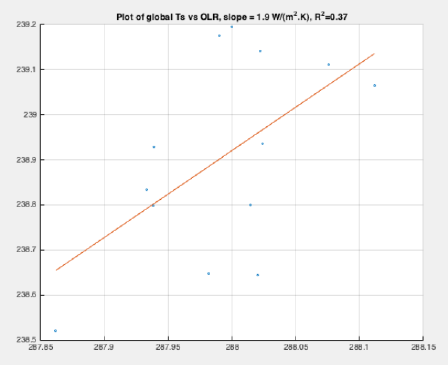
I am not quite sure why Steve C. used 3.6 as Planck Response, which is the consensus figure for clear sky samples. Here it would seem these are just global all sky data, so that the benchmark should be 3.3 by consensus terms. But ok, it only makes for a minor issue.

Way more important here are the common pitfalls with regression analyses. If you look closer onto the chart, you might realize there is a much larger interval on the y-scale (0.7) than on the x-scale (0.3). Also the grid is not square, but a bit wider than high. And although the numbers themselves, for temperature and radiation, are incidentally in comparable ranges, the x-scale relative to the y-scale, is stretched out by about 2.5 to 1.

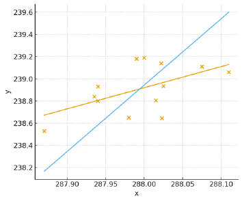
So I went through those 13 data points, estimated their values as good as possible from the graph, and typed them into excel. I wanted to see what it would look like without stretching the x-scale, but rather keep both scales in proportion. On top of that I added a 1.9W/m² regression line. It is hand drawn and only meant for illustration btw.

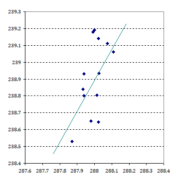
Yes, the regression is obviously wrong – it should be much steeper. I mean by using the wrong intervals on the x- or y-scale, you can make any scatter plot look either flat, or vertical. Equally you can make it appear well spread out, when it is actually mainly vertical, as it is in this instance. The adaptive scaling in excel, or similar, will only promote this deception. I played this little trick on the SoD data. Important: it is the same data, just different scales and aspect ratios.

The Plot, the Scatter and the Slope

Let us take a step back and look at the bigger picture. Below I show the SB law and how the result scales with temperature. I think it is very important to include the 0 point and have both scales at identical intervals. On top of that I highlighted the typical area of interest in terms of Earth science. There are those temperatures we tend to deal with and the according radiation figures, blackbody or not. Numerically you will have small scattering on the x- and large scattering on the y-scale, every single time.

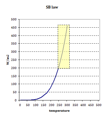
The numerical relation between temperature and radiation, as in the chart above, is naturally large with the Earth like temperature range. Any OLS (ordinary least squares) regression over such data sets will carry the same problem, thereby vastly underestimating the actual dOLR/dT_s relation. But there is a remedy for it, it is called TLS, or total least squares, the gold standard of linear regressions so to say. This illustration was taken Paster-Galan et al 2017² in the field of geology, a science where they actually seem to care doing proper regressions, and you would not be called a “geology denier” for doing so.

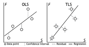
OLS is simply minimizing the vertical distance (squared) between the regression line and the data points. Ideally that vertical residual would stand rectangular to the regression line. The steeper the slope, the more the residual stands parallel to it, thereby turning the approach “blunt”, while it remains insensitive towards errors in x-values.

TLS on the other side minimizes the rectangular distance. As long as the numerical distribution is more or less horizontal, OLS and TLS will give similar results. If however the distribution is more vertical, meaning a small numerical spread on the x-scale but a large on the y-scale, OLS will be objectively wrong. I mean it could still be correct, if there was definitely no error in the describing variable, but practically that is barely ever so, and certainly not in the given context.

There is a simplistic way to check if an OLS regression gives a reasonable result - by flipping the axes. The x-values become y-values and vice verse. The reciprocal result should be at least similar to the previous result to validate it. In the above example that would be 1.9 vs. 6.33, meaning you can not trust the result and “the truth” will be somewhere in between. I am not statistician, but I do recall having learnt something like that in school. In this instance however, the higher figure will be much closer to the truth, just because the distribution is strongly vertical.

In fact this issue quickly started boiling in the comments to the linked SoD article, and rightfully so. One commenter pointed out the inverted regression would then give him 6.2W/m², thereby vastly overshooting the 3.6W/m² Planck Response, meaning a huge negative feedback. Of course the “discovery” as such went nowhere, because everyone assuming the data must be wrong. Well..

TLS on the other hand is “immune” to this problem, though it is not perfect either, as it is scale-sensitive, other than OLS. For instance, if you match body height vs. weight, the TLS result will depend on what metric you use. A metric cm/kg relation will give a materially different result than an imperial inch/pound relation. Yet this error will be relatively(!) small as compared to what an illicit OLS regression can do.

It might seem like there is no correct regression technique, because none gives the perfect result. However, that is naturally so with statistics. Statistics is the science of uncertainty, not providing certainty or a definite truth, but instead trying to contain said uncertainty. For that reason statistical analyses come along with plenty of “small print”, different parameters I mostly do not understand and get largely ignored anyway. These are meant to provide the context to what is just circumstantially true, more or less. Statistics give us perspectives, or views, which are relatively right, or relatively wrong.

However, of course that will not mean one could pick one arbitrary perspective of choice and then claim it was “the truth”, especially so if it is well documented that is circumstantially wrong. By (ab-)using standard OLS regressions on the dOLR/dT_s relation “climate science” consistently produces an error vastly understanding said relation. Considering there is the benchmark Planck Response, such statistical woes will constantly produce positive feedbacks that are just an artefact.

Some reanalysis

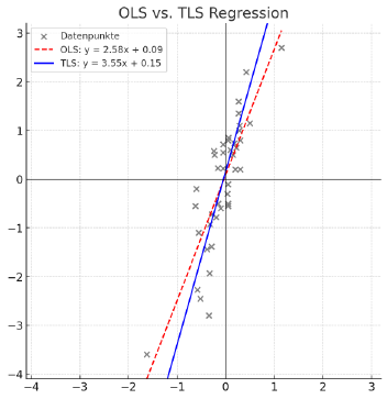
Regrettably there seems to be no online tool for TLS regressions. I dumped the SoD data into ChatGPT and other AIs, to sure up it would not just be a hallucination. ChatGPT calculated an OLS regression of 1.9, the same figure SoD claimed. So that would suggest I did a decent job with reading the data points from the chart. The TLS regression however yields 5.97! As expected it would be close to the inverted OLS result. If you assume a Planck Response of 3.6, that means a negative WV + LR feedback of -2.37W/m²/K based on satellite data!? A massive negative feedback right in front of us, and no one sees it. How could that be? The ChatGPT chart below shows the both regressions. The wrong OLS line in orange and the correct TLS result in blue.

And now it is not hard for me read your minds. You would think blue does not look right, rather orange does. Obviously what I say must be wrong, or ChatGPT (and others) miscalculated once more, which it often does. Also I am making the outlandish claim the science was all wrong, even too dumb to do regressions, based on dealing with the issue for just about a week!? What are the chances? Yet I will tell you, no, orange is wrong and blue is right, and the only reason you think else, lies in the original sin this chart incorporates. And it has fooled legions of scientists, not just with climate. Also I had multiple AI engines run over the data, with identical results btw.

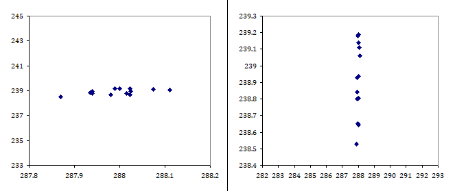
So let me do the magical trick and open your eyes. The whole problem disappears if we straighten out the chart, something I already pointed out with the excel chart above. If we use symmetric intervals on both axes, the point cloud reveals its true shape, without distortion. Remember, these are the very same data as above, we only synchronized the intervals.

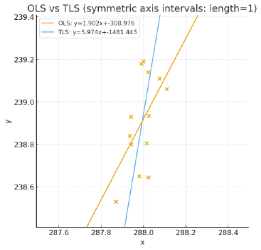
What you think now? Orange or blue, which regression is correct? Yes, it is definitely blue, it always was. The problem is as old as excel. Every time you make a chart with some data points, the program automatically fits the intervals to give maximum resolution - on both scales. In many instances that is perfectly fine and desirable. But it also distorts the shape of the scatter plot. When the distribution is highly vertical, as it is here, that distortion will make it look rather round and diffuse. Combine that with a simple OLS regression, and you will get a result that looks optically sound, but actually is completely wrong. The deception is perfect!

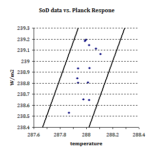
And just to provide yet another view, because I know most people would struggle with judging the validity if statistical analyses. In its core this is not complicated, a school child would easily understand it. Ask a child if the data plot in the chart below is steeper or flatter than the Planck Response, shown as black lines. Flatter means a positive-, steeper a negative feedback. You would need to turn a blind eye on this to assume feedbacks were positive, or that it was just a complicated academic statistical discussion. Rather it is bloody simple.

In “climate science” this blunder holds a decent share in the positive WV feedback delusion. Just because it is not the only problem with the “consensus scientific” papers on WV feedback, as they are already struck with other serious issues discussed before, does not make it any better, au contraire. But when it comes to makeshift plausibility checks, like with the SoD example, the gloves are off.

Spencer’s Regression

For instance we have this one article from Roy Spencer³, where he argues for low climate sensitivity.

Anyway, here is the result for 15 years of annual CERES net radiative flux variations and HadCRUT4 surface temperature variations, with the radiative flux lagged 4 months after temperature:
 
Fig. 1. Global, annual area averages of CERES-measured Net radiative flux variations against surface temperature variations from HadCRUT4, with a 4 month time lag to maximize correlation (flux after temperature).

Coincidentally, the 1.3 deg. C best estimate for the climate sensitivity from this graph is the same as we got with our 1D forcing-feedback-mixing climate model, and as I recently got with a simplified model that stores energy in the deep ocean at the observed rate (0.2 W/m2 average since the 1950s).

Again, the remaining radiative forcing in the 15 years of data causes decorrelation and (almost always) an underestimate of the feedback parameter (and overestimate of climate sensitivity). So, the real sensitivity might be well below 1.3 deg. C, as Lindzen believes. The inherent problem in diagnosing feedbacks from observational data is one which I am absolutely sure exists — and it is one which is largely ignored. Most of the “experts” who are part of the scientific consensus aren’t even aware of it, which shows how a small obscure issue can change our perception of how sensitive the climate system is.

This is also just one example of why hundreds (or even thousands) of “experts” agreeing on something as complex as climate change really doesn’t mean anything. It’s just group think in an echo chamber riding on a bandwagon.

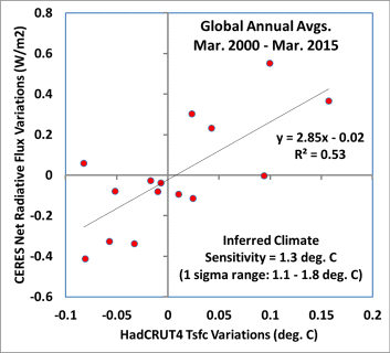
Spencer calculated, with OLS, a dOLR/dT_s relation of 2.85. Just let me clarify how he gets to a climate sensitivity of 1.3K from it. Assuming a Planck Response of 3.3W/m², you get 3.3 – 2.85 = 0.45W/m² for WVF. With a CO2 forcing of 1.1K, you could then calculate ECS = 1.1 / (1 - 0.45 / 3.3) = 1.27, or ~ 1.3K. Alternatively you can short cut it to 3.7/2.85 = 1.3. Arguably there would be no albedo feedback included in the proxy, so that ECS eventually should turn out higher.

The funny part is about the regression again. The chart given has a total interval of 1.4 on the y- and only 0.3 on the x-scale. The whole thing is badly distorted and that is the only reason his regression seems to fit. There is actually a pretty simplistic way to guess the regression of such a data plot, without using much math. All you have to do is to guess the extent of the data points on both scales. On the x-scale it might reach from -0.085 to +0.16, and -0.42 to +0.55 on the y-scale. Then (0.55+0.42)/(0.16+0.08) = 4. It is not precise and the sign you will have to guess, although that is usually not the problem. But it is still a hell lot better and more accurate, than falling for an illicit OLS regression on a vertical data plot.

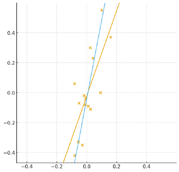
I dumped the whole chart into ChatGPT and asked to guess a TLS regression estimate. Result: ~4.5W/m²/K. But of course, being a perfectionist, I could not help to go a step further. You know, I need to be certain. So again I typed down the data points into excel and ran them through perplexity AI (I always check back on multiple AIs, just to be sure). The OLS regression resulted in 2.84, which is pretty close to the 2.85 Spencer names. My pixel work again was pretty accurate. The TLS regression however resulted in 5.22!!!

As 5.22 > 3.3, the data Spencer presents actually show a huge negative feedback, like -1.92. But he failed to see it, just because of the wrong regression – and “tricky” excel. Had he done the regression right, he would have ended up with an ECS of only 3.7 / 5.22 = 0.71K. Ok, that would still be without albedo feedback, but even with it, ECS would stay comfortably <0.8K.

Lindzen, Choi

Once you know what to watch out for, you find this blunder all over the place.  The next one is from Lindzen, Choi 2009⁴, plotting tropical dOLR/dSST. SST stands for sea surface temperature. The red dots and lines btw. reveal how I do these kind of reanalysis. Like this it is still not perfect, but it comes pretty close.

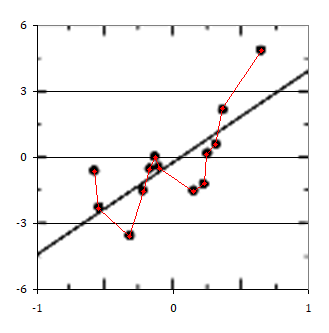
Chart and text indicate a slope of 4.23. My reanalysis yields 4.23 with the OLS regression (spot on) and 7.55 with the here appropriate TLS regression. While LC09 indeed argues a negative feedback, like 3.6(?) – 4.23 = -0.63W/m²/K, it is just long shot from what the data actually hold. 3.6 – 7.55 = -3.95W/m²/K!!!

A negative tropical feedback in the magnitude of -4W/m2 is certainly beyond imagination, even for “sceptical scientists”. But based on the data I have seen so far, it is absolutely consistent. The upper troposphere reacts very strongly to changes in SST in the tropics, warming or cooling by a factor of ~3! Only an increase of 2K in T_z yields a (neg.) temperature feedback of ~8W/m² (= ~(262^-260^4)*5.67e-8). The inner tropics specifically feature an abundance of high altitude clouds, lifting the emission altitude even further and making OLR more susceptible to changes in the lapse rate.

The problem with LC09, next to the regression, is that they obviously did not understand or reflect on the lapse rate. For one, the term lapse rate is not mentioned once in the paper, although it is the pivotal factor in the negative feedback they argue. For the other, instead they refer to their previously postulated “Iris hypothesis” as possible cause, which is wrong and pointless. It is hard to grasp someone like Lindzen would not get it, but well..

LC09 had a follow up, LC11⁵. While this paper at least mentions lapse rate feedback once, that instance only clarifies how L&C did not understand it:

In the models.. the long wave feedback appears to be positive, but it is not as great as expected for the water vapor feedback.. This is possibly because the so-called lapse rate feedback.. acting to cancel some of the TOA OLR feedback in current models

No, it is not just possibly so, but of course it is, because it has to be. And it is not just an alleged, “so called” lapse rate feedback, rather it is one fundamental thing, without which you just can not understand atmospheric physics. Although inexplicable to me, the wording, the circumstances, the alternative “Iris hypothesis” all show how Lindzen and Choi regrettably were just noobs in this regard.

The paper however does take a huge upturn when it comes to the regression issue:

“we show that simple regression methods used by several existing papers generally exaggerate positive feedbacks and even show positive feedbacks when actual feedbacks are negative..
but we see clearly that the simple regression always undere stimates negative feedbacks and exaggerates positive feedbacks”

Yep! It surprised me when I read the paper while writing this article. The regression issue did not go totally unnoticed. The strange thing is though, LC11 was written kind of in defense of LC09 to support the “outlandish” claim of negative feedbacks. The regression issue was not featured at all in LC09. It looks like this issue was just introduced to back up the previous paper, which is kind awkward. Really it would have deserved a display on its own right.

I mean, I can not blame them because I run into the same issue every single time. I start writing an article, try to make it short and on point, but inevitably I will turn a few stones on the way and find more notable stuff. The story then just keeps growing in an iterative process. It is simply how the epistemological cookie crumbles. And there is indeed more discussion on the subject, like by Gred Goodman⁶ or Nic Lewis⁷ on Judith Curry’s blog.

If you check out the discussion, you will see there is a lot of back- and forth on what might be the correct regression, and as I have stated above, there is no perfect one. However, they all seem to be unaware of the scale-distortion discussed above. If you manage to get over this issue and fix it, regressions become intuitively understandable. You can almost assess them with your bare eyes, it is then not complicated anymore. We kind of have a head start here owed to a richer, multi-dimensional view on the subject.

Chung et al 2010⁸

And then of course we also have it with the “consensus side”. Despite we already know how they got the all the feedback proxies wrong in multiple ways, I had to check if the regressions were another layer of failure. So here is the interannual chart from Chung et al 2010 (C10), with the data points identified.

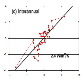
I have do say there will be a little bias with the y-values because the scales are not perfectly synchronized. However, that is just a deviation of ~0.05 in absolute terms, but relatively and in terms of the regression itself, that will have no impact. The data points themselves have been well identified with just minimal and non-systemic imprecisions. The only actual problem is that some data points might be doubles, impossible to identify.

If you take a closer look, something about this chart looks fishy. In the upper half there are almost no residuals to the right, but instead those on the left side look extremely dominant. That should not be possible. I do not know what this is, but it does not look like a regression. Either there is some data point outside the range of this graph, or they just drew a random line. Both instances would disqualify it. Even an illicit plain OLS regression should have a steeper slope here.

The reanalysis reveals some very interesting details. OLS is NOT 2.4, but 2.58, or rounded to one decimal 2.6. C10 has all other proxies in the 2 to 2.3 range. 2.6 then is an inconvenient figure, an outlier, something you might want to hide away, and that might be exactly what they did. The inverted OLS regression yields 3.65 btw.

The (correct!) TLS regression tells a totally different story anyway. The result is 3.55W/m²/K, basically on par with the clear sky Planck Response of 3.6, meaning no feedback at all. Given the circumstances that is amazing. By sampling for clear skies, these data feature a far larger spread in Ts than ever occurred. Also clouds are the primary factor in “communicating” the negative lapse rate feedback - more on that on that in a separate article. The point is, these data have already been illicitly “optimized” to turn an actual negative feedback into the opposite. And yet they fail to make it into the positive territory, if it is not for an equally illicit regression.

Also it will not even need to have complex statistical methods to reveal the problem, as above a simple comparison between the scatter plot and Planck Response should do the trick. Note that with clear skies emissions will be larger than a typical ~240W/m², even more so if the measured data are latitude restricted due to non-polar orbits. The Planck Response is 3.6W/m²/K here, as in C10.

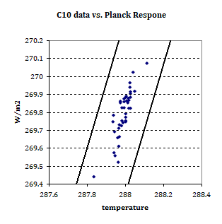
It is not just the optical impression, but also TLS regression telling us the slopes are more or less identical. On top of that, if it were not for the two outliers, which we know are artefacts due to clear sky sampling, the TLS slope of the remaining points is 4.7! That too is easily optically verifiable, I mean not the exact number, but one can see the scatter plot is then clearly steeper than the PR benchmark.

Conclusio

So yes, feedbacks are negative, the evidence is all over place, and has always been. All the narrow minded, insufficient intellects manage to not see it, for the always the same reason: tunnel vision and lack of resolution. It is the nature of great intellect to not be restricted to expertise, but rather to have the choice between maximum width of view AND as much focus as needed. It is the combination of both capabilities to break the apparent walls of epistemology. Maybe compare it to a predator like a cat, which does not just bite its prey, but also shakes it to break it. It is the combination of factors.

The key to understanding regressions is proper data visualization with symmetric aspect ratios. Once you understand this, you can virtually guess the slope of a linear regression without even having to rely on the complex mathematics behind it. The error margin by guessing will typically be far smaller than the “regression dilution” generated from illicit applications of standard OLS regressions.

The lack of this knowledge, or the unawareness if you will, is the reason why “climate science” believes simple OLS regressions were fine, why feedbacks were positive, climate sensitivity was high and even relevant, why we have an “energy transformation” destroying the west while handing over absolute power to China, and why there are now inevitable wars coming up to settle the so generated polito-tectonic tensions.

It is equally the reason why the marginal discussion of the subject on the “critical side” has barely advanced, and definitely not taken off. If you see this as a highly academic question over the proper regression technique, this would exclude anyone except statisticians. Naturally then some non-professionals might take note, but without standing they will shrug their shoulders and move on. But this blunder is as real as tangible.

¹https://scienceofdoom.com/2015/07/20/clouds-water-vapor-part-ten-data-iii-annual-ts-vs-olr/

²https://www.researchgate.net/publication/312869256_Bootstrapped_total_least_squares_orocline_test_A_robust_method_to_quantify_vertical-axis_rotation_patterns_in_orogens_with_examples_from_the_Cantabrian_and_Aegean_oroclines

³https://www.drroyspencer.com/2015/07/15-years-of-ceres-versus-surface-temperature-climate-sensitivity-1-3-deg-c/

⁴https://agupubs.onlinelibrary.wiley.com/doi/full/10.1029/2009GL039628

⁵https://www.researchgate.net/publication/227314777_On_the_observational_determination_of_climate_sensitivity_and_its_implications

⁶https://judithcurry.com/2016/03/09/on-inappropriate-use-of-least-squares-regression/

⁷https://judithcurry.com/2019/10/18/gregory-et-al-2019-unsound-claims-about-bias-in-climate-feedback-and-climate-sensitivity-estimation/

⁸https://agupubs.onlinelibrary.wiley.com/doi/full/10.1029/2009GL041889