Last year, when Gavin Schmidt explained the CO2 problem in six easy steps¹ on the realclimate blog, I could not help to hint towards the surface emissivity problem. You know, while the consensus largely assumes an emissivity of unity, it is rather about 0.91 in reality. This blunder alone produces a chain reaction of more severe consequences, like overstating the GHE, getting the attribution wrong, overstating climate sensitivity and messing up climate models in a way that no super computer will ever fix.

Gavin was so kind to respond: “Not really sure why you think this, but LW emissivity for different surfaces is well-known and is represented in most (all?) GCMs and in the energy budget described above.”

Notably he did not dispute, though neither endorse, the fact that surface emissivity is about 0.91. How do we know it is? I explained it here on this site and we have some notable references giving identical results²³⁴. So it is known physics and hard to argue with, except for some details possibly.

On the other side it is neither credible these emissivities could have been properly accounted for, be it in models or elsewhere. An obvious hint to it is already the “earth energy budget” diagram posted by Gavin. A 398.2W/m2 in surface emissions are impossible to attain, unless you assume an emissivity of 1. So the suggestion is extremely odd. Not just is Gavin the head of NASA climate research, he is also a leading figure in climate modelling. Him only just assuming the models should have it right, is hard to grasp.

This kind of triggered me. I already knew about the whole mess, but I was curious to learn how it came to it. You know it is all about the dialectic approach, trying see things from the other side, from different perspectives. And what I discovered is just an amazing story. A fairy tale, a comedy starring some of the worlds “leading experts”. You just could not make this up.

Wilber et al⁵

It all starts with a paper called “Surface Emissivity Maps for Use in Satellite Retrievals of Longwave Radiation” by Wilber et al, 1999 (W99). As the title suggests this paper had a specific scope. If you want to monitor surface temperatures, you can do this with a satellite measuring radiation within the atmospheric window. This comes with a couple of issues since some of that radiation will be attenuated by the atmosphere, and obviously you will need a clear sky. Most of all however, since radiation is a function of temperature AND emissivity, you will need information on the emissivity of the surface you are looking at. Only then you can make a reasonable estimate on what the temperature is. That is where the idea of, or rather the need for, emissivity maps originates.

Algorithms developed for the CERES processing use surface emissivity to determine the longwave radiation budget at the Earth's surface. As a consequence, surface emissivity maps were needed as soon as the CERES instrument began taking measurements.

If the authors had restricted themselves to this scope, there probably would not have been much trouble. Some inaccuracies there and there could have had an impact on satellite temperature data, if the paper was actually used for that, but otherwise no. While the author’s skill level was rather insufficient for this alone, their ambitions reached far further. This “bridge too far” came in the shape of providing “broadband emissivity” figures, meaning the whole spectral emissivity.

In general, the laboratory measurements spanned the wavelength range of 2-16 µm. At wavelengths greater than 16 gm, the emissivity was extrapolated, i.e., the measured emissivity´in the interval closest to 16 µm was replicated to fill the remaining bands where data were not available.

Since they had NO DATA within the far-IR range, which accounts for about 50% of total emissions, they just guessed. Of course this is completely pointless, because why would you suggest any random figures, when you simply do not have the information? And if someone wants to, or rather feels like he needs to guess, he is free to do so anyway and will not require a guess-suggestion?! Only the idea of doing so is totally childish.

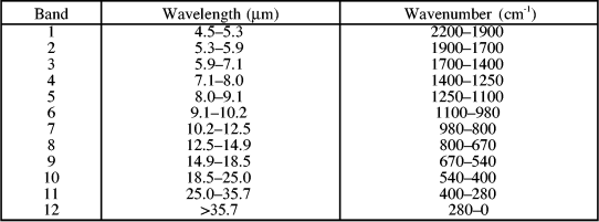
Another completely useless “tool” the paper uses are so called “Fu-Liou” bands. For the sake of semantic clarity I will refer to them as fool-you bands. These introduce the amazing technology of splitting up the spectrum into 12 arbitrary bands, without need, and without scope. In fact this is a typical pattern of bureaucrats doing pointless stuff, just for feeling obliged to do anything, without having the brain to so something meaningful. So, here are your fool-you bands:

And as if this was not bad enough, things go steeply downhill from there on. Next the paper categorizes 18 different kinds of surface, with water being number 17. Again, this is fine from a bureaucratic perspective, but in reality water covers 70% of the planet and materially is by far the most important surface type. Maybe they should have paid a little more attention to it, as this could have saved them, and us all, from the blunders to come.

The present study assumes the transmittance (Tz) of the surface to be zero. Applying Kirchhoff's Law which states that the absorptance (Az) is equal to the emittance (ez) under conditions of thermodynamic equilibrium yields a straightforward relationship between reflectance (Rz.) and emissivity

This is one of the few things I will agree with. Because emissivity = 1 – reflectivity we can just as well show the data as reflectivity, which promotes clarity and presentability. Given I have already presented the data on the reflectivity of water (or emissivity respectively), the most logical step is to compare these with what Wilber et al present. Please try not to laugh!

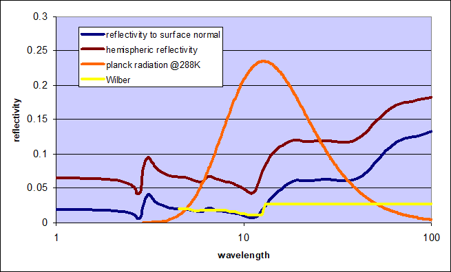
Up to fool-you band 8 (14.9µm) they got it roughly right, although at a very poor resolution. From there on however their assumptions were no good, to say at least. Unexpectedly the reflectivity of water strongly increases in the far-IR range, something you could not guess, if you, well, just guess. So their super smart extrapolation technique turned out to be a complete failure. Next to being use- and senseless from the beginning, I should add.

Of course the authors were well aware of having insufficient data and so they pointed out that additional research would be required. Given the paper was published in 1999 and we are writing 2023, it might seem a bit unfair to laugh at their ignorance. One would expect a lot more data becoming researched and known in the meanwhile. In fact I took the data from the website refractiveindex.com, and that one took it from Hale, Querry 1973(!!!)⁶. In other words, high resolution and high quality data on the emissivity of water was available for at least 26 years, when Wilber et al published their patchwork.

To deal with these readily available data they would have been required to dive a little deeper, next to properly searching the scientific literature. They would have had to deal with Fresnel equations, understand how water is not a Lambertian radiator, or most importantly distinguish between emissivity to surface normal and hemispheric. In other words, they would have had to deal with physics, which can be time consuming and complicated. Instead they just skipped it.

If at this point you might think science could not sink any lower, I have a little surprise for you! In Appendix B Wilber et al give us the “precise” data on the emissivities of different surface types, among which of course water. Those are summarized in this stupid table below..

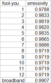
As you can easily see, the values from fool-you band 8 were simply “extrapolated” into the further bands, but that is a blunder we already discussed. Way more interesting here is the broadband emissivity they calculated. Notably it is higher than any of the fool-you bands meant to cover the whole emission spectrum. So what was their technique?

To calculate a broadband emissivity from the band-average emissivities, the Planck function was used to energy weight each of the 12 band-average emissivities. The weighted values were then combined into a broadband emissivity.

That is perfectly logical, in fact it is just what I did. The problem is rather, that regardless of the weighting, there is no way the average can yield a value higher or lower than the range of values within the sample. Imagine you would have 5 numbers between 1 and 3, and you were told the average of these was 8!? This is not going to work, and the same thing applies for the broadband emissivity W99 claims. The average over all those fool-you bands is well beyond the range of all of them. It is a mistake so obvious and stupid, you might best ignore it. A typo kind of thing, you know.

In fact, when trying to forensically replicate it, I would assume when doing the averaging they had fool-you bands 9 to 12 at 1, which was their default number for a lot of other surface types. In this case the weighted average I calculated is 0.9905, pretty close to what the paper claims. It is wrong anyway, so it will not matter.

What matters instead is the question, why I am discussing a peer reviewed paper so rotten and stupid, that it jeopardizes the concept of peer review itself. By no means, if peer review would guarantee an absolute minimum of quality and integrity, such a paper would ever have been published. Obviously peer review is about something else. And what matters even more is the influence this paper had on “climate science”, brace for impact!

Trenberth et al 2008⁷

While Wilber et al 1999 is barely a household name in the “climate science” community, Trenberth et al 2008 (T08) “Earth’s Global Energy Budget” definitely is. Nonetheless even their take on surface emissivity is a bit creative, to say at least. In the “Spatial and temporal sampling” box they first of all use KT97⁸, that is themselves, as a reference for the blackbody assumption. But instead of dealing with this issue and considering a more realistic surface emissivity, they turned the opposite way.

They picked up a rational thought, that is relative to the arithmetic average, the real temperature distribution will mean more emissions, as they are a logarithmic function by the power of 4. For instance if we split up Earth into two hemispheres, one at 273K and the other at 303K, then the average is still 288K. The blackbody emissions however then would amount to 396.4W/m2
( = (273^4 + 303^4)/2*5.67e-8 ) instead of just 390W/m2. In this way you can reasonably argue somewhat higher surface emissions, and a somewhat larger GHE as logical consequence.

Next they present this formula to calculate the deviation in actual emissions due to departures from the global mean both in space and time. I am not sure the formula makes actually sense, but the brackets are definitely misplaced. Oh peer review, where are thou?

T⁴ =T_g⁴(1 +  6[T´/T_g)²+(T´/T_g)⁴]

The ratio T´/Tg is relatively small. For 1961-90, Jones et al. (1999) estimate that Tg is 287.0 K, and the largest fluctuations in time correspond to the annual cycle of 15.9°C in July to 12.2°C in January, or 1.3%. Accordingly, the extra terms are negligible for temporal variations owing to the compensation from the different hemispheres in day versus night or winter versus summer. However, spatially time-averaged temperatures can vary from -40°C in polar regions to 30°C in the tropical deserts. With a 28.7-K variation (10% of global mean) the last term in (2) is negligible, but the second term becomes a nontrivial 6% increase.

Indeed, if you apply the formula as it was meant, not as it was written, with the arbitrarily chosen 10% variation, you get a 6% increase in emissions. Instead of 390W/m2 with an average 288K, you could now argue 390 * 1.06 = 413.4W/m2 in surface emissions, and the GHE would grow to almost 175W/m2, way more than they aimed for. Consequently they lowered the average surface temperature from 288K in KT97 to a more realistic 287K.

The problem with that is, a 6% is completely off the charts. One needs to consider that most of the planet, about 70%, is covered by water with temperature spread from 0 to 30°C. This is a very moderate spread and has almost no impact (~0.6%). A significant spread is restricted to land which covers only about 30% of the surface, limiting its impact as well. If you account for it properly, you will get a 2.5% increase at best. With a 287K in average surface temperature, you could argue up to 394W/m2 in surface emissions (=287^4*5.67e-8 * 1.025), not more.

T08 then goes on to argue they had actually used a model to calculate emissions of 396.4W/m2. Notably, if the 6% deviation was correct, this would mean an average surface temperature of only 285K (=((396.4/1.06)/5.67e-8)^0.25). In this way they are somehow contradicting their own notion. Anyway, all this is still based on the blackbody assumption. It looks like all these not so reasonable theoretical considerations they named, were only meant to provide some headroom to push both surface emissions and the magnitude of the GHE. The practical implication there of course being climate sensitivity eventually.

Things become spicy when they finally try to justify their blackbody assumption:

The surface emissivity is not unity, except perhaps in snow and ice regions, and it tends to be lowest in sand and desert regions, thereby slightly offsetting effects of the high temperatures on LW upwelling radiation. It also varies with spectral band (see Chedin et al. 2004, for discussion). Wilber et al. (1999) estimate the broadband water emissivity as 0.9907 and compute emissions for their best-estimated surface emissivity versus unity. Differences are up to 6 W m-2 in deserts, and can exceed 1.5 W m-2 in barren areas and shrublands

Yes, there it is. T08 uses the trash paper W99 as a reference to support their blackbody assumption and quote the infamous 0.9907. Adding insult to injury, they even ignore that 1% deviation. This detail alone would have reduced emissions by 4W/m2, meaning they would barely progress from the 390W/m2 KT97 named, jeopardizing the politically motivated attempt to enlarge the GHE. And so the emissivity of water grew from (the real) 0.91 to 0.99 due to sheer incompetence, and from 0.99 to 1, because who cares? Science at its finest!!!

Excursion: a stupid perspective

Now there is another stupid thought ventilated in the quote above and it is very much alive to this day. How would surface emissions even matter? The perspective is that most of the emissions will get absorbed by the atmosphere anyway. If only like 10% of surface emissions pass through the atmospheric window, then a 1% deviation in surface emissions would only result in 0.1% change in actual emissions TOA. Again, who cares? From this perspective it appears to be a non-issue. Let me add this quote from Huang et al:

When the surface spectral emissivity dataset is used in the atmospheric radiative transfer calculation, its impacts on global-mean clear-sky OLR and all-sky OLR are both nonnegligible. Moreover, the spatial pattern of such impact is not uniform. Comparing to the case of blackbody ocean surface as used in current numerical models, taking spectrally dependent ocean surface emissivity into account will reduce the OLR computed from the radiation scheme. Such reduction of OLR changes with latitude, ranging from ~0.8 Wm-2 in the tropics to ~2 Wm-2 in the polar regions. Over lands, the largest differences are seen over desert regions. Specifically, changes in OLR due to the inclusion of surface spectral emissivity are most discernible in the mid-IR window as well as the "dirty window" in the far IR, even for the globally averaged differences. The discernible difference in the far-IR dirty window is supporting evidence why the far-IR observations are urgently needed for a complete and accurate understanding of the Earth radiation budget.

This is giving the right answers (probably) to the wrong question. If everything else remained the same, then this might be true. In reality however, the GHE is defined as the difference between surface emissions and emissions TOA. So for every single W/m2 of less surface emissions, the GHE shrinks equally by one W/m2. Given surface emissions are larger than the GHE, percentage wise this means a much larger shrink. For instance surface emissions may drop from 395W/m2 to only 355W/m2, while the GHE at the same time shrinks from 155W/m2 to 115W/m2.

The magnitude of the GHE will directly impact the attribution to the individual greenhouse agents. The cake so to say can only be distributed once, and if gone, there is nothing left to distribute. Because of this surface emissivity directly impacts the significance of individual GHGs, some more, some less. As pointed out, WV is most severely affected.

On top of that there is an undeniable logic “climate science” refuses to comprehend. What is true for the GHE, is equally true for the enhanced GHE, because it is physically the same thing. This logical necessity can easily be demonstrated with modtran, this time from spectral sciences⁹. It is important only to use the mid-latitude summer model, as all others are defunct. The following table gives the emissions TOA depending on CO2 concentration and albedo. With the albedo we are effectively changing emissivity in the model, with emissivity = 1 – albedo. To reproduce these results let me provide the exact parameters¹⁰. You need to read “upward diffuse (100km)” btw.

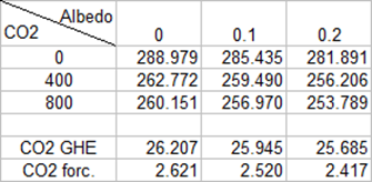
As we can see surface emissivity has a direct impact on CO2 forcing. On top of that the same would be true for WV feedback, and any other GHGs. In this scenario however, due to the strong WV concentration, the effect is still attenuated. The whole thing becomes way more obvious, if we remove other GHGs (and thus overlaps).

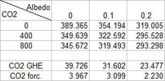
As a matter of fact the variable surface emissivity directly affects

-    the magnitude of the greenhouse effect
-    the attribution of the greenhouse effect to individual greenhouse gases
-    climate sensitivity
-    emissions top of the atmosphere

With the first three variables the effect is naturally enhanced and huge, while it is attenuated and small with the last. The stupid perspective is to only look at the last variable and argue there was not much of a problem.

The proper perspective

It is easy to see the bigger problem here. There are a lot of vital variables depending on surface emissivity. But these variables are already hard coded in the models and will not change by only changing surface emissivity. In this way the model output is isolated from the real physical impacts. Ironically a simple model like modtran can instead, at least partially, replicate these dependencies. The only variable allowed to change are emissions TOA, which is of minor significance. And that again makes people believe there were no other implications. Apart from that, there are most certainly no provisions to account for the complexities of a non-Lambertian radiator as water is. Again Huang et al:

The offline evaluation in this study only estimates the impact of surface spectral emissivity on the TOA radiation budget assuming everything else remains unchanged. It does not include any changes of atmosphere, thermodynamically or dynamically, in response to such changes of lower boundary conditions in radiative transfer and, consequently, the changes in radiation budget and in atmospheric-column radiative cooling.

Let them eat cake!

We are talking about a conceptual misunderstanding. If people have no bread, let them eat cake. This is a perfectly reasonable suggestion, if you assume there was some misallocation of resources within bakeries. They produced too much cake and too little bread. If people adept to supply and eat more cake, the problem is fixed. In reality however the problem will rather be a general lack of food, and people who can not afford bread, will certainly not afford cake. “Climate science” here takes the message at face value, without realising the implications!

Let us look at the bigger picture

W99 focused on a specific scope and the authors thought they could provide more information, like broadband emissivity, just on the way. They were completely unaware of the complexity of the subject. Anyway the paper should never have been published given all its fallacies. K08 on the other hand wanted to confirm earlier assumptions, and likely even seeked to expand the GHE for idiologic reasons. To them W99 must have looked like a useful reference to support their otherwise baseless assumption of surface emissivity being unity. And so this unholy alliance of incompetence and bias gave us this graph (and many alike)..

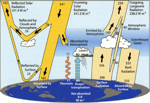
With an attitude towards quality assurance in the shape of “the science is settled” and anyone contradicting is a “science denier”, there is naturally zero awareness of the problem. And even if someone came up and pointed to it, his job as a climate scientist might soon be in question. For this reason it also remains unclear if authors like Huang et al did not understand the implications of their otherwise reasonable work, or whether they just not dared to be more explicit. For instance it is obvious how their hemispheric spectral emissivity chart of water translates into a numerical emissivity of 0.91. However, they did not name it.

Back to Gavin’s question

“Not really sure why you think this, but LW emissivity for different surfaces is well-known and is represented in most (all?) GCMs and in the energy budget described above.”

1. First of all because you do not even know LW surface emissivity, as NASA’s “earth energy budget” proves
2. Because we know about the blunders in W99 and T08 making you believe you knew
3. Because we know about the implications of actual surface emissivity, and we see these implications are nowhere accounted for
4. Because we get some “hints” from Huang et al: “To the best of our knowledge, this study is the first attempt to construct a global surface spectral emissivity dataset over the entire LW spectrum”, or “Comparing to the case of blackbody ocean surface as used in current numerical models..”
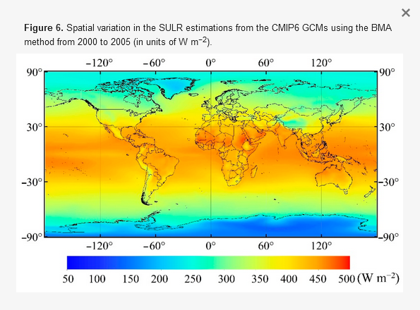
5. Because of this chart taken from Xu et al 2021¹¹. Sorry for relying on this external source, rather than extracting the data right from GCMs (which I have not done, or managed to do yet respectively). What this chart indicates are emissions in the 470W/m2 region for the warmest tropical ocean segments. We know the tropical ocean surface barely exceeds 30°C. At this temperature, with an emissivity of 1, you get 479W/m2 in emissions, but only 436W/m2 with an emissivity of 0.91. So CGMs must use an emissivity of unity, or something very close to it.

Conclusion

I think this example shows very well how things go wrong, and why they go wrong in “climate science”. It is a combination of incompetence and hubris in an environment where criticism is considered denial. In a politically biased atmosphere, we have the perfect cocktail of ingredients that are all toxic to science. Even the idea something fruitful could come out of this, is purely illusive. While such blatant failure provides an abundance of leverage to the “critical side”, which desperately seeks to falsify the orthodoxy, it fails to take advantage, because its protagonists are at least as incompetent.

Also this example shows how Gavin Schmidt, one of the most reputated climate scientists, will not understand the problem, even if you point the finger right onto it. He can not even imagine there was one, given all the resources that were poured into the research, the thousands of “experts”, the peer reviews and the backslapping within the community. He would probably think of himself as a sharp minded critical thinker, while in reality he is highly confirmation biased.

All these pillars the “science” is based on exist in a safe space, in part because it is politically desired and in part because the lack of a critical AND capable opposition. This article shall demonstrate what is possible, once these obstacles are overcome. A reasonably sharp minded analysis shatters these pillars with ease, not because of any super-powers, but because they were rotten from the start.

But this is far more than just a showpiece on how things go wrong, rather the surface emissivity issue has direct consequences on the most basic questions of “the science”. The greenhouse effect, the role of water vapor and climate sensitivity are all vastly exaggerated due to this blunder. The implications are so severe, that it invalidates “climate science” as whole, demanding a restart of the modelling process. And it is just one blunder out of many.

¹https://www.realclimate.org/index.php/archives/2022/07/the-cos2-problem-in-six-easy-steps-2022-update/

²Beahr, Stephan 2011 „Heat and Mass Transfer” - link.springer.com/book/10.1007/978-3-642-20021-2

³Huang et al 2016 - journals.ametsoc.org/downloadpdf/journals/atsc/73/9/jas-d-15-0355.1.pdf

⁴Feldman et al 2014 - www.pnas.org/doi/10.1073/pnas.1413640111

⁵Wilber et al - https://www.researchgate.net/publication/24315801_Surface_Emissivity_Maps_for_Use_in_Retrievals_of_Longwave_Radiation_Satellite

⁶https://pubmed.ncbi.nlm.nih.gov/20125343/

⁷https://journals.ametsoc.org/downloadpdf/journals/bams/90/3/2008bams2634_1.pdf

⁸https://journals.ametsoc.org/view/journals/bams/78/2/1520-0477_1997_078_0197_eagmeb_2_0_co_2.xml

⁹http://modtran.spectral.com/modtran_home

¹⁰Mode: radiance; atmosphere model: mid-latitude summer; water column: 3635.9; ozone column: 0.33176; CO: 0.15; CH4: 1.8; ground temperature: 294.2; aerosol model: rural; visibility: 23.0; sensor altitude: 99km; sensor zenith: 180 deg; spectral units: wavenumbers; spectral range: 250.0 to 2500.0; resolution: 5cm-1; 2nd scenario: water column, ozone column, CO, CH4 set to zero

¹¹https://www.mdpi.com/2072-4292/13/21/4464